This material has been adapted from material by Fergus Cooper and others from the "Essential Mathematics" module at the Doctoral Training Centre, University of Oxford.
This course material was developed as part of UNIVERSE-HPC, which is funded through the SPF ExCALIBUR programme under grant number EP/W035731/1
Systems of differential equations 2
Learning outcomes
Be able to analyse non-linear systems in multiple dimensions
Understand how to simplify the form of a system using parameter re-scaling
Understand how to use properties of a system to simplify the set of equations
Understand the concept of a phase plane
Be able to identify nullclines of a non-linear system
Be able to plot the phase plane of a non-linear system
Be able to plot the phase plane of a non-linear system using matplotlib in Python
YouTube lecture recording from October 2020
A recording of this lecture from October 2020; the material has changed a little since.
System simplification
Recap
So far we have looked at systems of first order, linear ODEs in two dimensions
These systems can be solved analytically
3 methods of solving systems of first order ODEs
Diagonalisation extends to N-dimensional systems
Plan
Aim to look at systems of first order, nonlinear ODEs in more dimensions
How we go about modelling a problem
Simplifying systems of ODEs
Reducing number of parameters
Reducing number of equations
Phase plane analysis
System simplification: rescaling
This predator-prey model is in dimensional terms and contains 5 parameters.
dTdNdTdP=rN(1−KN)−bNP,=ebNP−mP.
r: prey intrinsic growth rate
K: prey carrying capacity (bound to logistic growth)
b: predation rate
e: conversion efficiency
m: per capita predator mortality rate
If we substitute
N=θn
P=ϕp
T=τt
where n,p,t are nondimensional, and θ, ϕ and τ is a typical values for N, P and T.
Note that, when we are re-scaling time:
dTd=dtddTdt=τ1dtd.
The original equations are:
dTdNdTdP=rN(1−KN)−bNP,=ebNP−mP.
And, after rescaling, we have:
τθdtdnτϕdtdp=θrn(1−Kθn)−bnpθϕ,=ebnpθϕ−mpϕ.
Note that θ, ϕ and τ are arbitrary values for scaling N, P, and T.
dtdndtdp=τ(rn(1−Kθn)−bnpϕ),=τ(ebnpθ−mp).
After rearranging we note that choosing θ=K will remove the parameter K from the equations.
Choosing τ=1/m (or τ=1/r) will remove a further parameter.
n˙p˙=(mrn(1−n)−mbϕnp),=(mebpKn−p).
ϕ=m/b gives the two parameter system:
n˙p˙=(mrn(1−n)−np),=(mebpKn−p),
where we have shifted the groups of parameters to only two places.
We could make it more obvious that there are only two "tuning dials" by writing it as:
n˙p˙=v1n(1−n)−np,=p(v2n−1),
System simplification: conservation
Consider a chemical system where a product is formed from a substrate via an intermediate complex involving an enzyme.
S+Ek−1⇌k1C→k2P+E
This system can be written as a system of 4 ODEs for s,e,c,p which describe the concentrations of S,E,C and P:
In the previous example it may be known that the rate of conversion to complex (from k1 and k−1) is much faster than the degradation of complex into product (rate k2).
If this is the case then we can assume that the concentration of C arrives at some level c∗ (a quasi-steady state) and then moves very slowly.
This means that we have used conservation and quasi-steady state to go from a 4-dimensional system (s,e,c,p) to a two-dimensional approximation which captures some of the behaviour.
Two dimensions are good because we can plot their behaviour on a phase plane diagram.
Phase planes and nullclines
A system of nonlinear ODEs may have more than one fixed point (or may have none).
Finding fixed points in two-dimensional systems is aided by nullclines.
An x-nullcline is a line where x˙=0 and a y-nullcline is a line where y˙=0.
(These are straight lines in the linear case.)
For example:
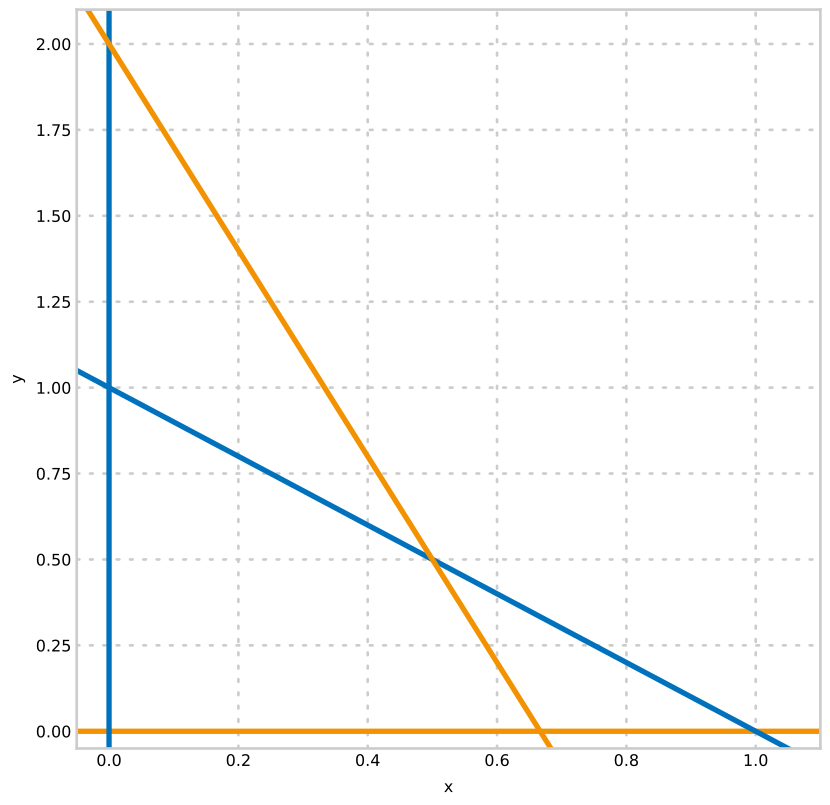
x˙y˙=x(1−x)−xy,=2y(1−2y)−3xy,
has x-nullclines at x=0 and 1−x−y=0; and y-nullclines at y=0 and 2−3x−y=0.
Nullcline intersections give us the fixed points.
Nullclines can be annotated to give the direction (and magnitude) of the non-zero derivative.
Plot of the nullclines
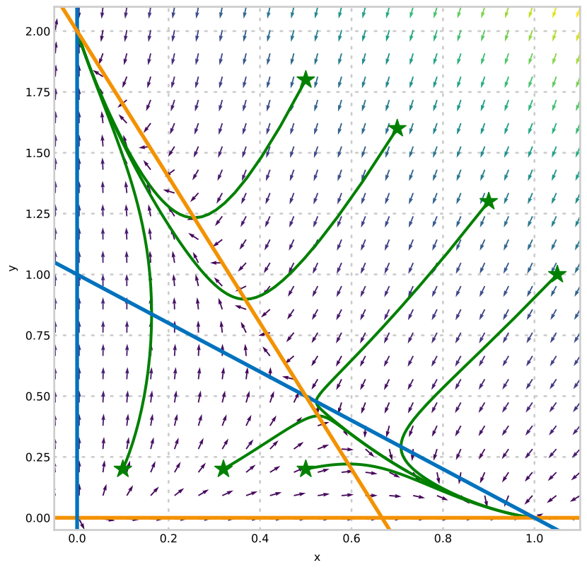
Plot of the phase plane
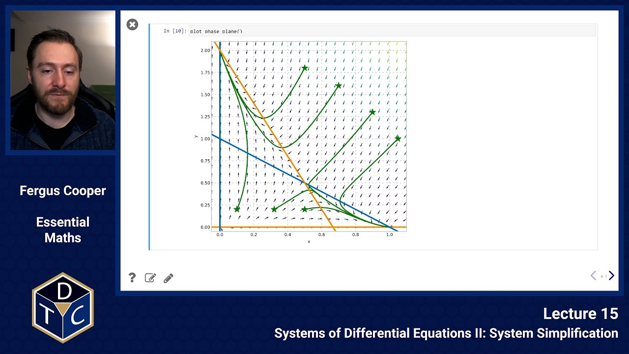
The nullclines allow us to add arrows demonstrating the flow direction, and by following the arrows we can sketch the behaviour of solutions (green lines).
The arrows can only cross the x-nullclines vertically, and the y-nullclines horizontally.
Python code to plot the phase plane
import numpy as np
from matplotlib import pyplot as plt
from scipy.integrate import solve_ivp
defdX_dt(t, X):return np.array([ X[0]*(1.- X[0])- X[0]*X[1],2.*X[1]*(1.-X[1]/2.)-3*X[0]*X[1]])defplot_phase_plane(): plt.figure(figsize=(10,10)) init_x =[1.05,0.9,0.7,0.5,0.5,0.32,0.1] init_y =[1.0,1.3,1.6,1.8,0.2,0.2,0.2] plt.plot(init_x, init_y,'g*', markersize=20)for v inzip(init_x,init_y): X0 = v # starting point sol = solve_ivp(dX_dt,(0,10), X0, t_eval=np.linspace(0,10,100)) plt.plot(sol.y[0], sol.y[1], lw=3, color='green')# plot nullclines x = np.linspace(-0.1,1.1,24) y = np.linspace(-0.1,2.1,24) plt.hlines(0,-1,15, color='#F39200', lw=4, label='y-nullcline 1') plt.plot(x,1- x, color='#0072bd', lw=4, label='x-nullcline 2') plt.vlines(0,-1,15, color='#0072bd', lw=4, label='x-nullcline 1') plt.plot(x,2-3*x, color='#F39200', lw=4, label='y-nullcline 2')# quiverplot - define a grid and compute direction at each point X, Y = np.meshgrid(x, y)# create a grid DX = X*(1-X)- X*Y # evaluate dx/dt DY =2*Y*(1- Y/2.0)-3*X*Y # evaluate dy/dt M =(np.hypot(DX, DY))# norm growth rate M[ M ==0]=1.# avoid zero division errors plt.quiver(X, Y, DX/M, DY/M, M) plt.xlim(-0.05,1.1) plt.ylim(-0.05,2.1) plt.xlabel('x') plt.ylabel('y')
Summary
Simplification
Rescaling to dimensionless quantities
Conservation
Quasi-steady state approximation
Nullclines are a powerful way of finding steady states and phase flow
Introductory problems
For more practice, an AI tool can write new problems like the ones below.
Ask it for problems of the same type and difficulty, or for problems set in your own field.
For example, you could ask it to "write five chemistry problems on fixed points and rescaling, at the level of these ones".
Work them on paper first, then ask the tool to check your answers and to explain any step you are unsure of.
Introductory problems 1
Find the fixed points of the following linear systems:
x˙=x+3y,y˙=−6x+5y;
x˙=x+3y+4,y˙=−6x+5y−1;
x˙=x+3y+1,y˙=−6x+5y.
At a fixed point x˙=0 and y˙=0, so in each case we solve a pair of simultaneous equations.
x+3y=0 gives x=−3y.
Substituting into −6x+5y=0 gives 18y+5y=0, so y=0 and x=0.
The fixed point is (0,0).
Multiply the first equation by 6 and add it to the second:
(6x+18y+24)+(−6x+5y−1)=23y+23=0
So, y=−1, and then x=−4−3y=−1.
The fixed point is (−1,−1).
In the same way, (6x+18y+6)+(−6x+5y)=23y+6=0, so y=−6/23, and then x=−1−3y=−5/23.
The fixed point is (−5/23,−6/23).
Introductory problems 2
Find the fixed points of the following nonlinear systems:
x˙=−4y+2xy−8y˙=4y2−x2;
x˙=y−x2+2,y˙=2(x2−y2).
y˙=0 gives x2=4y2, so x=2y or x=−2y.
Substitute each into x˙=0.
x=2y: −4y+4y2−8=0, so y2−y−2=(y−2)(y+1)=0.
This gives y=2, x=4 and y=−1, x=−2.
x=−2y: −4y−4y2−8=0, so y2+y+2=0.
This has no real solutions, because 12−4×2<0.
The fixed points are (4,2) and (−2,−1).
x˙=0 gives y=x2−2, and y˙=0 gives y=x or y=−x.
y=x: x2−x−2=(x−2)(x+1)=0, which gives (2,2) and (−1,−1).
y=−x: x2+x−2=(x+2)(x−1)=0, which gives (−2,2) and (1,−1).
There are four fixed points: (2,2), (−1,−1), (−2,2) and (1,−1).
Main problems
Main problems 1
Consider the chemical reaction network:
⟶k0Ak−1⇌k1B⟶k2
Write down the system of two linear ODEs which describe the evolution of the concentrations of A and B in this system under the law of mass action.
Find the ratio of concentrations of A and B for which this system is in steady state: that is the concentrations do not change over time.
Let a=[A] and b=[B].
A is produced at the constant rate k0, turns into B at rate k1a, and is made from B at rate k−1b.
B is removed at rate k2b.
So,
dtdadtdb=k0−k1a+k−1b=k1a−k−1b−k2b
In steady state db/dt=0, so k1a=(k−1+k2)b, and
ba=k1k−1+k2
We can also find the concentrations themselves.
Adding the two equations gives k0−k2b=0, so b∗=k0/k2, and then a∗=k0(k−1+k2)/(k1k2).
Main problems 2
Consider the reversible enzyme reaction:
S+Ek−1⇌k1Ck−2⇌k2P+E
Verify the Haldane relation, which states that when the reaction is in equilibrium,
sp=k−1k−2k1k2,
where p and s are the concentrations of P and S, respectively.
Let s, e, c and p be the concentrations of S, E, C and P.
By mass action,
dtdsdtdp=−k1se+k−1c=k2c−k−2pe
In equilibrium the concentrations do not change, so both are zero:
k1se=k−1candk2c=k−2pe
The first gives c=k1se/k−1.
Substituting this into the second,
k−1k1k2se=k−2pe
The enzyme concentration e cancels, so
sp=k−1k−2k1k2
(We can check that dc/dt=k1se−k−1c−k2c+k−2pe is then zero too.)
Main problems 3
The population of a host, H(t), and a parasite, P(t), are described approximately by the equations:
dTdH=(a−bP)H,dTdP=(c−HkP)P,H>0,
where a,b,c,k are positive constants.
By a suitable change of scales show that these equations may be put in the simpler form
y˙=(1−x)y,x˙=αx(1−yx),
where α=c/a.
Sketch the phase flow across the following lines:
y=x;
x=0;
y=0;
x=1;
y=βx, for β greater than and less than 1.
As in the lecture, let T=τt, P=θx and H=ϕy, where τ, θ and ϕ are scales still to be chosen, so that d/dT=(1/τ)d/dt.
Then
τϕy˙=(a−bθx)ϕyandτθx˙=(c−ϕykθx)θx
so
y˙=τ(a−bθx)yandx˙=τ(c−ϕykθx)x
Choosing τ=1/a and θ=a/b gives y˙=(1−x)y, and
x˙=(ac−bϕykx)x=acx(1−bcϕkayx)
Finally, choosing ϕ=ka/(bc) gives x˙=αx(1−x/y), with α=c/a.
Now the flow across each line.
x and y are populations, so we only need x≥0 and y>0.
On y=x, x˙=0 (this is an x-nullcline), so the flow crosses it vertically.
y˙=(1−x)x, so the flow is upwards for x<1 and downwards for x>1.
On x=0, x˙=0 and y˙=y>0, so the flow is up the y axis.
With no parasites, the hosts grow exponentially.
On y=0, y˙=0 (a y-nullcline).
The equations are not defined on the line itself, because of x/y, but just above it x/y is very large, so x˙ is large and negative and the flow moves sharply to the left.
With almost no hosts, the parasites die out.
On x=1, y˙=0 (a y-nullcline), so the flow crosses it horizontally.
x˙=α(1−1/y), so the flow is to the right for y>1 and to the left for y<1.
On y=βx, x˙=αx(1−1/β) and y˙=βx(1−x).
For β>1 (above the line y=x) the flow is to the right, and for β<1 (below it) the flow is to the left.
In both cases it is upwards for x<1 and downwards for x>1.
Putting these together, the flow goes clockwise around the point (1,1), where the nullclines y=x and x=1 cross (we find out what happens there in the next lecture).
For example, with α=1:
import numpy as np
from matplotlib import pyplot as plt
alpha =1x, y = np.meshgrid(np.linspace(0.01,2.5,30), np.linspace(0.01,2.5,30))xdot = alpha * x *(1- x / y)ydot =(1- x)* y
plt.streamplot(x, y, xdot, ydot, color='grey')plt.plot([0,2.5],[0,2.5], color='#0072bd', label='x-nullcline y = x')plt.axvline(0, color='#0072bd', label='x-nullcline x = 0')plt.axvline(1, color='#F39200', label='y-nullcline x = 1')plt.axhline(0, color='#F39200', label='y-nullcline y = 0')plt.xlabel('x (parasites)')plt.ylabel('y (hosts)')plt.legend()
Main problems 4
Consider a lake with some fish attractive to anglers.
We wish to model the fish-angler interaction under the following assumptions:
the fish population grows logistically in the absence of fishing;
the presence of anglers depresses the fish growth rate at a rate jointly proportional to the size of the fish and angler populations;
anglers are attracted to the lake at a rate directly proportional to the number of fish in the lake;
anglers are discouraged from the lake at a rate directly proportional to the number of anglers already there.
Write down a mathematical model for this situation, clearly defining your terms.
Use a suitable scaling to show that a non-dimensionalised version of the model is
x˙=rx(1−x)−xy,y˙=βx−y
Let F(T) be the number of fish and A(T) the number of anglers at time T.
Then
dTdFdTdA=aF(1−KF)−bFA=cF−eA
where all the constants are positive:
a is the growth rate of the fish, and K is the largest number of fish the lake can support (its carrying capacity);
b measures how quickly anglers catch fish;
c measures how strongly the fish attract anglers;
e is the rate at which anglers are discouraged and leave.
As in the lecture, let F=θx, A=ϕy and T=τt, so that d/dT=(1/τ)d/dt.
Then
x˙y˙=τax(1−Kθx)−τbϕxy=ϕτcθx−τey
Choosing θ=K, τ=1/e and ϕ=e/b gives
x˙=eax(1−x)−xyandy˙=e2bcKx−y
which is the model given, with r=a/e and β=bcK/e2.
Main problems 5
Consider the reaction chain
S⟶k1I⟶k2P
in which a substrate is converted to a product through a short-lived intermediate.
Write down the system of three ODEs for s, i and p under the law of mass action.
Show that s+i+p is constant, and use this to eliminate p.
Suppose the second step is much faster than the first (k2≫k1).
Use a quasi-steady state for i to find i∗ in terms of s, and hence an approximate equation for dp/dt.
Explain why the rate at which P is made depends only on k1 in this approximation.
Each step uses up one species and makes the next, so
dtdsdtdidtdp=−k1s,=k1s−k2i,=k2i.
Adding the three equations,
dtd(s+i+p)=−k1s+k1s−k2i+k2i=0
so s+i+p=T, where T is a constant: the total amount of material.
Then p=T−s−i, and the system reduces to the two ODEs for s and i.
If k2≫k1, the intermediate is used up almost as soon as it is made, so i quickly reaches a quasi-steady state.
Solving di/dt=0:
k1s−k2i∗=0⇒i∗=k2k1s
This is small, because k1/k2 is small, and it moves slowly with s.
Substituting it into the equation for p,
dtdp=k2i∗≈k1s
In this approximation, every molecule of I is turned into P almost straight away, so P is made as fast as I is made, which is k1s.
The first step is the slow one, so it limits the rate of the whole chain.
This is often called the rate-limiting step.