OxRSE Training

Linear Systems

YouTube lecture recording from October 2020

The following YouTube video was recorded for the 2020 iteration of the course. The material is still very similar:

Our aim is to solve systems of equations of the form:

$\displaystyle \frac{{\rm d}y_i}{{\rm d}t} = f_i(y_1,\ldots,y_n,t),$

for

\displaystyle i=1,\ldots,n

Let us first consider the simplest form: a

2\times2

linear system

\begin{align*} \frac{{\rm d}x}{{\rm d}t} &= ax+by,\\ \frac{{\rm d}y}{{\rm d}t} &= cx+dy. \end{align*}

Motivation

In order to understand these systems, we must first understand coupled linear systems.

Recap of eigenvalues

\displaystyle A = \left(\begin{matrix} 1 & 1\\2 & 0 \end{matrix}\right)

import sympy as sp
A = sp.Matrix([[1, 1],[2, 0]])
A.eigenvals()

$\displaystyle \left\{ -1 : 1, \ 2 : 1\right\}$

Recap of eigenvectors

\displaystyle A = \left(\begin{matrix} 1 & 1\\2 & 0 \end{matrix}\right)

A.eigenvects()

$\displaystyle \left[ \left( -1, \ 1, \ \left[ \left[\begin{matrix}- \frac{1}{2}\\1\end{matrix}\right]\right]\right), \ \left( 2, \ 1, \ \left[ \left[\begin{matrix}1\\1\end{matrix}\right]\right]\right)\right]$

Recap of diagonalisation

Recall that, for a matrix

A

with eigenvectors

\mathbf{v}_1

and

\mathbf{v}_2

, and eigenvalues

\lambda_1

and

\lambda_2

, we can write a matrix of eigenvectors:

P = \left(\begin{matrix} \mathbf{v}_1 & \mathbf{v}_2 \end{matrix}\right)

. Then:

$\displaystyle A = P \left(\begin{matrix} \lambda_1 & 0 \\ 0& \lambda_2 \end{matrix}\right) P^{-1}$

(This is also true for general

n \times n

matrices.)

In our example,

$P = \left(\begin{matrix} -\frac{1}{2} & 1 \\ 1& 1 \end{matrix}\right),\qquad\lambda_1 = -1,\qquad\lambda_2=2.$

Coupled ODEs

For coupled system of first order linear differential equations of the form

\begin{align*} \frac{{\rm d}x}{{\rm d}t} &= ax+by,\\ \frac{{\rm d}y}{{\rm d}t} &= cx+dy. \end{align*}

we have three methods of analysing them mathematically:

Turn them into one second order equation (if we can solve second order!)
Divide one by other, to get one equation independent of $t$
Perform matrix diagonalisation (extends to $n \times n$ problems)

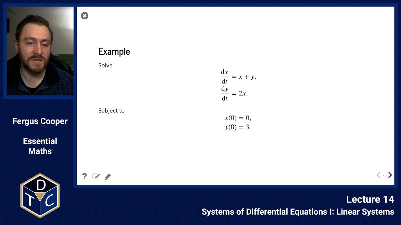
Example

Solve

\begin{align*} \frac{{\rm d}x}{{\rm d}t} &= x+y,\\ \frac{{\rm d}y}{{\rm d}t} &= 2x. \end{align*}

Subject to

\begin{align*} x(0) &= 0,\\ y(0) &= 3. \end{align*}

Method 1: Second order

We start with:

\begin{align*} \frac{{\rm d}x}{{\rm d}t} &= x+y,\\ \frac{{\rm d}y}{{\rm d}t} &= 2x. \end{align*}

We can convert that into a second order equation:

\frac{{\rm d}^2x}{{\rm d}t^2} = \frac{{\rm d}x}{{\rm d}t} + \frac{{\rm d}y}{{\rm d}t} = \frac{{\rm d}x}{{\rm d}t} + 2x \quad \quad\implies \quad\quad \boxed{\frac{{\rm d}^2x}{{\rm d}t^2} = \frac{{\rm d}x}{{\rm d}t} + 2x}

Method 2: eliminate $t$

We start with:

\begin{align*} \frac{{\rm d}x}{{\rm d}t} &=& x+y,\\ \frac{{\rm d}y}{{\rm d}t} &=& 2x. \end{align*}

Then, dividing:

\frac{{\rm d}y}{{\rm d}x} = \frac{ \quad \frac{{\rm d}y}{{\rm d}t} \quad }{ \frac{{\rm d}x}{{\rm d}t} } \quad \quad\implies \quad\quad \boxed{\frac{{\rm d}y}{{\rm d}x} = \frac{2x}{x+y} }

Method 3: diagonalisation

Let

\displaystyle \mathbf{v}=\left(\begin{matrix}x\\y\end{matrix}\right),

then

\frac{{\rm d}x}{{\rm d}t} = x+y,\quad \frac{{\rm d}y}{{\rm d}t} = 2x, \quad \implies \quad \boxed{\frac{{\rm d}\mathbf{v}}{{\rm d}t} = A\mathbf{v},}

where

\displaystyle A = \left(\begin{matrix} 1 & 1\\2 & 0 \end{matrix}\right).

Substitute

$\displaystyle A = P \left(\begin{matrix} \lambda_1 & 0 \\ 0 & \lambda_2 \end{matrix}\right) P^{-1}.$

then

$\displaystyle \frac{{\rm d}\mathbf{v}}{{\rm d}t} = P \left(\begin{matrix} \lambda_1 & 0 \\ 0 & \lambda_2 \end{matrix}\right) \left( P^{-1}\mathbf{v} \right)\qquad$

$\displaystyle \frac{{\rm d}}{{\rm d}t}(P^{-1} \mathbf{v}) = \left(\begin{matrix} \lambda_1 & 0 \\ 0 & \lambda_2 \end{matrix}\right) \left( P^{-1}\mathbf{v} \right)$

We can now introduce a new variable

\displaystyle \;\mathbf{z} = \left(\begin{matrix} z_1 \\ z_2\end{matrix}\right) = P^{-1} \mathbf{v}\;

so that:

$\displaystyle \frac{{\rm d}\mathbf{z}}{{\rm d}t} = \left(\begin{matrix} \lambda_1 & 0 \\ 0 & \lambda_2 \end{matrix}\right) \mathbf{z}.$

But now, because the matrix is diagonal, the system is no longer coupled. The first equation only involves

z_1

and the second only involves

z_2

, so we can solve each one individually:

$\displaystyle \frac{{\rm d}z_1}{{\rm d}t} = \lambda_1 z_1 \qquad\implies\qquad z_1(t) = A\,e^{\lambda_1 t}$ > $\displaystyle \frac{{\rm d}z_2}{{\rm d}t} = \lambda_2 z_2 \qquad\implies\qquad z_2(t) = B\,e^{\lambda_2 t}$

Finally, we can substitute

z_1

and

z_2

back in terms of

x

and

y

to find the solution to the original coupled system:

We have

$\displaystyle \mathbf{z} = \left(\begin{matrix} z_1 \\ z_2\end{matrix}\right) \quad = \quad P^{-1} \mathbf{v} \quad = \quad \frac{1}{3}\left(\begin{matrix} -2 & 2 \\ 2& 1 \end{matrix}\right) \left(\begin{matrix} x \\ y\end{matrix}\right) \quad = \quad \left(\begin{matrix} A\,e^{\lambda_1 t} \\ B\,e^{\lambda_2 t}\end{matrix}\right)$

Rearranging, we now have two equations relating

x

and

y

$\displaystyle -2x + 2y = C\,e^{\lambda_1 t}$ > $\displaystyle 2x + y = D\,e^{\lambda_2 t}$

where

C=3A

and

D=3B

. Using our initial conditions,

\,x(0)=0\,

and

\,y(0)=3\,

we find

C=6

and

D=3

Finally, solving the simultaneous equations, we have a solution:

$\displaystyle x(t) = -e^{\lambda_1 t} + e^{\lambda_2 t}$ > $\displaystyle y(t) = 2e^{\lambda_1 t} + e^{\lambda_2 t}$

Summary

Three methods to analytically solve systems of linear first order ODEs
Best method depends on the system and what you need to ask about it

Introductory problems

Introductory problems 1

Find the general solution to the following system of ODEs:

$\displaystyle \def\dd#1#2{{\frac{{\rm d}#1}{{\rm d}#2}}} \dd{x}{t} = x, \quad\text{and}\quad \dd{y}{t}=y.$

Sketch the form of the solution in the

x,\,y

plane, using arrows to indicate where the solution moves over time.

Introductory problems 2

Take the general decoupled linear system

$\displaystyle \def\dd#1#2{{\frac{{\rm d}#1}{{\rm d}#2}}} \dd{x}{t} = ax, \quad\text{and}\quad \dd{y}{t} = by.$

Integrate the two equations separately to solve for $x$ and $y$ in terms of $t$ .
If you start at $t=0$ , $x(0)=0$ , $y(0)=0$ what happens to the solution over time?
If you start at a general position $x(0)=x_0$ , $y(0)=y_0$ what happens to the solution as $t\rightarrow\infty$ ?
- What if $a$ and $b$ are both negative?
- What if only one of $a$ or $b$ is negative? What if either $x_0$ or $y_0$ is negative?
Either by eliminating $t$ from the original equations or by eliminating $t$ from your solutions to part 1., find a general solution of the system. (Why not try both methods?)
Sketch this solution for
- $\quad a>0,\;\;b>0,\;\;a=b$
- $\quad a>0,\;\;b<0,\;\;a=-b$ .

Main problems

Main problems 1

By reformulating the following system as one first order equation (i.e eliminating

t

), find the general solution to:

$\displaystyle \def\dd#1#2{{\frac{{\rm d}#1}{{\rm d}#2}}} \dd{x}{t} = -y, \quad\text{and}\quad \dd{y}{t} = x.$

Sketch the form of the solutions in the

x,\,y

plane.

Main problems 2

Again by eliminating

t

and reformulating the system as one first order equation, find the general solution to the following system of ODEs:

$\displaystyle \def\dd#1#2{{\frac{{\rm d}#1}{{\rm d}#2}}} \dd{x}{t} = y, \quad\text{and}\quad \dd{y}{t} = x.$

Sketch the form of the solutions in the

x,\,y

plane.

Main problems 3

Find the eigenvalues and two independent eigenvectors

\mathbf{v}_{1}

and

\mathbf{v}_{2}

of the matrix

$\displaystyle A = \left(\begin{array}{cc} 1 & 4 \\ 1 & 1 \end{array} \right)$ .

Put the vectors $\mathbf{v}_{1}$ and $\mathbf{v}_{2}$ as the columns of a $2\times 2$ matrix $P$ . Find $P^{-1}$ and show (by calculation) that $P^{-1}AP$ is diagonal. What are the entries of this matrix? What do they correspond to?
Find the general solution of the system $\displaystyle \def\dd#1#2{{\frac{{\rm d}#1}{{\rm d}#2}}} \dd{x}{t} = x+4y, \quad\text{and}\quad \dd{y}{t} = x + y$ .
Find the particular solution subject to $x(0)=0$ and $y(0)=2$ .
Sketch the trajectory (the $x(t),\,y(t)$ coordinates over time) in the $x,\,y$ plane.
- Draw the eigenvectors $\mathbf{v}_{1}$ and $\mathbf{v}_{2}$ on the same figure.
- What happens as $t\rightarrow \infty$ ?
- What about $t\rightarrow -\infty$ ?
- What is $\displaystyle \def\dd#1#2{{\frac{{\rm d}#1}{{\rm d}#2}}} \dd{y}{x}$ at a general point on the $y$ -axis?

Extension problems

Extension problems 1

The force on a damped harmonic oscillator is

\displaystyle \def\dd#1#2{{\frac{{\rm d}#1}{{\rm d}#2}}} f = -k x - m \nu \dd{x}{t}

, where

x

is a displacement,

k>0

is a spring force constant,

m>0

is the mass and

\nu>0

is the strength of the damping.

Use Newton's 2nd law of motion to write down an equation for the acceleration $\displaystyle \def\ddd#1#2{{{{\rm d}^2#1}\over{\d{#2}^2}}} \def\d#1{{\rm d}#1} \ddd{x}{t}$ .
Make the substitution $\displaystyle \def\ddd#1#2{{{{\rm d}^2#1}\over{\d{#2}^2}}} \def\d#1{{\rm d}#1} \def\dd#1#2{{\frac{{\rm d}#1}{{\rm d}#2}}} y=\dd{x}{t}\;\left(\text{and hence }\dd{y}{t} = \ddd{x}{t}\right)$ to obtain a system of two first-order linear ODEs.

Systems of differential equations 1