Systems of differential equations 3: OxRSE Training

YouTube lecture recording from October 2020

A recording of this lecture from October 2020; the material has changed a little since.

Phase planes and stability

Recap from previous parts

2-D linear systems can be solved analytically
Eigenvalues are important
Some larger systems can be simplified
Phase planes, nullclines and fixed points allow us to understand the behaviour

Example from previous lecture

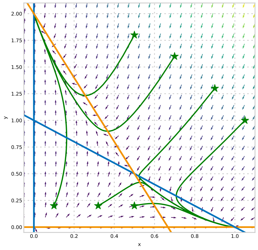
\begin{aligned} \dot{x} &= x(1-x) -xy,\\ \dot{y} &= y\left(2-y\right) - 3xy. \end{aligned}

Linear ODEs for understanding nonlinear

The decoupled ODE system

\begin{aligned} \dot{x} = \frac{dx}{dt} &= \lambda_1 x,\\ \dot{y} = \frac{dy}{dt} &= \lambda_2 y, \end{aligned}

has a fixed point or steady state where

\dot{x}=\dot{y}=0

, at the origin.

Solutions look like

x=Ae^{\lambda_1 t}

and

y=Be^{\lambda_2 t}

and thus grow exponentially or shrink exponentially depending on the values of

\lambda_1

and

\lambda_2

\lambda_1 < 0

and

\lambda_2 < 0

then all the flow is towards the fixed point. If

\lambda_1

\lambda_2

is positive then some flow will be driven away (towards infinity).

Adding in a constant (inhomogeneous) component shifts the fixed point away from the origin. Where is the fixed point of

\begin{aligned} \dot{x} &= \lambda_1 x + 10,\\ \dot{y} &= \lambda_2 y + 10? \end{aligned}

Coupling the system has the effect of altering the principle directions over which the exponential terms apply (changing the basis).

This means that the homogeneous linear system

\begin{aligned} \dot{x} &= a x + b y,\\ \dot{y} &= c x + d y, \end{aligned}

has a fixed point at the origin. The long-term growth or shrinkage of solutions over time is determined by the eigenvalues of the matrix

A = \begin{pmatrix} a & b \\ c & d \end{pmatrix}

More generally, the inhomogeneous linear system

\begin{aligned} \dot{x} &= a x + b y + p,\\ \dot{y} &= c x + d y + q, \end{aligned}

can be written

\left(\begin{array}{c} \dot{x} \\ \dot{y} \end{array}\right) = \left(\begin{array}{cc} a & b \\ c & d \end{array}\right) \left(\begin{array}{c} x \\ y \end{array}\right) + \left(\begin{array}{c} p \\ q \end{array}\right).

It has a fixed point at

\left(\begin{array}{c} x \\ y \end{array}\right) = -\left(\begin{array}{cc} a & b \\ c & d \end{array}\right)^{-1} \left(\begin{array}{c} p \\ q \end{array}\right).

The long-term growth or shrinkage of solutions over time is again determined by the eigenvalues of the matrix.

General nonlinear system steady states

A more general two-dimensional nonlinear system is

\begin{aligned} \dot{x} &= f(x,y),\\ \dot{y} &= g(x,y), \end{aligned}

where

f

and

g

can be any functions whatever.

We can write a polynomial (Taylor) expansion for the system when it is close to a fixed point

(x^*, y^*)

for which

f(x^*,y^*)=g(x^*,y^*)=0

\begin{aligned} \dot{x} &= f(x^*,y^*) + \frac{\partial f}{\partial x}(x-x^*) + \frac{\partial f}{\partial y}(y-y^*) + \ldots,\\ \dot{y} &= g(x^*,y^*) + \frac{\partial g}{\partial x}(x-x^*) + \frac{\partial g}{\partial y}(y-y^*) + \ldots \end{aligned}

So, close to the fixed point:

\def\arraystretch{1.8}\left(\begin{array}{c} \dot{x} \\ \dot{y} \end{array}\right) \approx \left(\begin{array}{cc} \frac{\partial f}{\partial x} & \frac{\partial f}{\partial y} \\ \frac{\partial g}{\partial x} & \frac{\partial g}{\partial y} \end{array}\right) \left(\begin{array}{c} x-x^* \\ y-y^* \end{array}\right).

This means that (really close to the fixed point) we can approximate with a linear system. The eigenvalues

\lambda_1

\lambda_2

of the matrix

\def\arraystretch{1.8}J = \left(\begin{array}{cc} \frac{\partial f}{\partial x} & \frac{\partial f}{\partial y} \\ \frac{\partial g}{\partial x} & \frac{\partial g}{\partial y} \end{array}\right)

will determine if a small perturbation away from

(x^*, y^*)

will decay or grow.

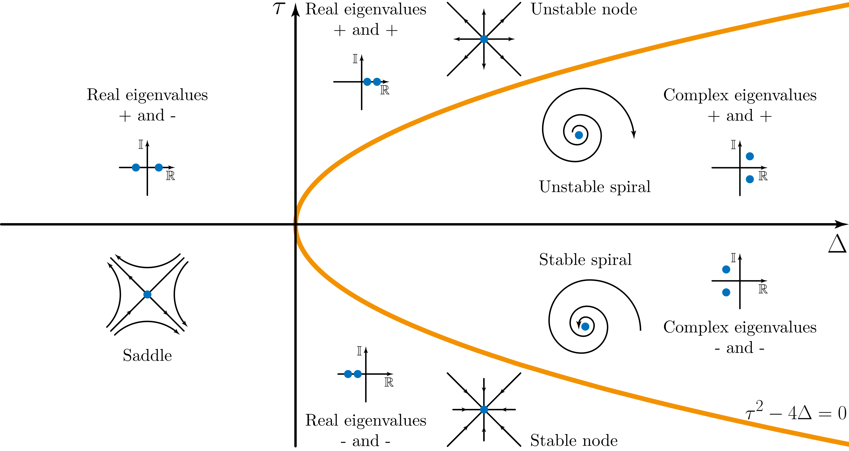
Steady state classification

\def\arraystretch{1.8}J = \left(\begin{array}{cc} \frac{\partial f}{\partial x} & \frac{\partial f}{\partial y} \\ \frac{\partial g}{\partial x} & \frac{\partial g}{\partial y} \end{array}\right)

$\lambda_1<\lambda_2<0$ : stable node
$\lambda_1=\lambda_2<0$ : stable star
$\lambda_1>\lambda_2>0$ : unstable node
$\lambda_1=\lambda_2>0$ : unstable star
$\lambda_1<0<\lambda_2$ : saddle (or hyperbolic) point, unstable
Complex $\lambda$ : spiral (with real part determining stability)
Imaginary $\lambda$ : neutral (solution cycles round fixed point)

The presence of negative eigenvalues determines whether a steady state is physically viable.

Eigenvalues of $J$

\def\arraystretch{1.8}|J-\lambda I| = \left| \begin{array}{cc} \frac{\partial f}{\partial x}-\lambda & \frac{\partial f}{\partial y} \\ \frac{\partial g}{\partial x} & \frac{\partial g}{\partial y}-\lambda \end{array}\right| = \left(\frac{\partial f}{\partial x}-\lambda\right)\left(\frac{\partial g}{\partial y}-\lambda\right)-\frac{\partial f}{\partial y}\frac{\partial g}{\partial x}

So eigenvalues

\lambda

satisfy

\lambda^2 - \lambda\left(\frac{\partial f}{\partial x} + \frac{\partial g}{\partial y}\right) + \frac{\partial f}{\partial x}\frac{\partial g}{\partial y} - \frac{\partial f}{\partial y}\frac{\partial g}{\partial x},

\lambda^2 - \lambda\tau + \Delta \quad \text{where} \quad \tau=\text{Trace}(J) \quad \text{and} \quad \Delta = \text{Det}(J)

Phase diagram showing different behaviour given the eigenvalues

Example system

\begin{aligned} \dot{x} &= x(1-x) -xy &&= f(x),\\ \dot{y} &= y\left(2-y\right) - 3xy &&= g(x). \end{aligned}

What are the nullclines?
What are the fixed points?
What is the stability of the fixed points?

Calculate the Jacobian

\def\arraystretch{1.8}J = \left(\begin{array}{cc} \frac{\partial f}{\partial x} & \frac{\partial f}{\partial y} \\ \frac{\partial g}{\partial x} & \frac{\partial g}{\partial y} \end{array}\right) = \left(\begin{array}{cc} -2x-y+1 & -x \\ -3y & -3x-2y+2 \end{array}\right)

(0,0)

J_{(0,0)} = \left(\begin{array}{cc} 1 & 0 \\ 0 & 2 \end{array}\right)

\left|\begin{array}{cc} 1-\lambda & 0 \\ 0 & 2-\lambda\end{array}\right|\quad\implies\quad\lambda_1 = 1, \quad \lambda_2 = 2 \qquad\text{(unstable)}

(1/2,1/2)

\def\arraystretch{1.8}J_{(1/2,1/2)} = \left(\begin{array}{cc} -\frac{1}{2} & -\frac{1}{2} \\ -\frac{3}{2} & -\frac{1}{2} \end{array}\right)

\def\arraystretch{1.8}\left|\begin{array}{cc} -\frac{1}{2}-\lambda & -\frac{1}{2} \\ -\frac{3}{2} & -\frac{1}{2}-\lambda\end{array}\right|\quad\implies\quad\lambda_\pm = \frac{1}{2} \pm \frac{\sqrt{3}}{2} \qquad\text{(saddle)}

(1,0)

J_{(1,0)} = \left(\begin{array}{cc} -1 & -1 \\ 0 & -1 \end{array}\right)

\left|\begin{array}{cc} -1-\lambda & -1 \\ 0 & -1-\lambda\end{array}\right|\quad\implies\quad\lambda_1 = \lambda_2 = -1 \qquad\text{(stable)}

(0,2)

J_{(0,2)} = \left(\begin{array}{cc} -1 & 0 \\ -6 & -2 \end{array}\right)

\left|\begin{array}{cc} -1-\lambda & 0 \\ -6 & -2-\lambda\end{array}\right|\quad\implies\quad\lambda_1 = -1, \quad \lambda_2 = -2 \qquad\text{(stable)}

If we now look again at the phase plane, after having calculated the stability of the fixed points, we can see that the arrows move towards the stable fixed points, and away from the unstable ones.

Summary

Eigenvalues tell us about the behaviour of linear systems
Eigenvalues tell us about the stability of nonlinear systems

Introductory problems

For more practice, an AI tool can write new problems like the ones below. Ask it for problems of the same type and difficulty, or for problems set in your own field. For example, you could ask it to "write five epidemiology problems on classifying steady states, at the level of these ones". Work them on paper first, then ask the tool to check your answers and to explain any step you are unsure of.

Introductory problems 1

Each matrix below is the Jacobian at a fixed point. Find its trace, determinant and eigenvalues, and classify the fixed point.

\begin{gathered} \text{(a)}\ \left(\begin{array}{cc} -3 & 0 \\ 0 & -1 \end{array}\right); \qquad \text{(b)}\ \left(\begin{array}{cc} 3 & 1 \\ 1 & 3 \end{array}\right); \qquad \text{(c)}\ \left(\begin{array}{cc} 1 & 2 \\ 2 & 1 \end{array}\right); \\ \text{(d)}\ \left(\begin{array}{cc} -1 & -2 \\ 2 & -1 \end{array}\right); \qquad \text{(e)}\ \left(\begin{array}{cc} 0 & 1 \\ -4 & 0 \end{array}\right) \end{gathered}

As in the lecture, the eigenvalues satisfy

\lambda^2 - \tau\lambda + \Delta = 0

, where

\tau

is the trace and

\Delta

is the determinant.

(a) $\tau = -4$ and $\Delta = 3$ , so $\lambda^2 + 4\lambda + 3 = (\lambda + 1)(\lambda + 3) = 0$ . The eigenvalues $\lambda = -1$ and $-3$ are both negative, so this is a stable node.
(b) $\tau = 6$ and $\Delta = 9 - 1 = 8$ , so $\lambda^2 - 6\lambda + 8 = (\lambda - 2)(\lambda - 4) = 0$ . The eigenvalues $\lambda = 2$ and $4$ are both positive, so this is an unstable node.
(c) $\tau = 2$ and $\Delta = 1 - 4 = -3$ , so $\lambda^2 - 2\lambda - 3 = (\lambda - 3)(\lambda + 1) = 0$ . The eigenvalues $\lambda = 3$ and $-1$ have opposite signs, so this is a saddle (unstable).
(d) $\tau = -2$ and $\Delta = 1 + 4 = 5$ , so $\lambda^2 + 2\lambda + 5 = 0$ and
$\lambda = \frac{-2 \pm \sqrt{4 - 20}}{2} = -1 \pm 2i$
The eigenvalues are complex with a negative real part, so this is a stable spiral.
(e) $\tau = 0$ and $\Delta = 4$ , so $\lambda^2 + 4 = 0$ and $\lambda = \pm 2i$ . The eigenvalues are purely imaginary, so this is neutral: solutions cycle round the fixed point.

Notice that a negative determinant always gives a saddle, because then the two eigenvalues multiply to give a negative number.

Introductory problems 2

The system

\dot{x} = x - xy, \qquad \dot{y} = x^2 - y

has fixed points at

(0, 0)

(1, 1)

and

(-1, 1)

. Find the Jacobian, evaluate it at each fixed point, and classify each one.

With

f = x - xy

and

g = x^2 - y

J = \left(\begin{array}{cc} \frac{\partial f}{\partial x} & \frac{\partial f}{\partial y} \\ \frac{\partial g}{\partial x} & \frac{\partial g}{\partial y} \end{array}\right) = \left(\begin{array}{cc} 1 - y & -x \\ 2x & -1 \end{array}\right)

At $(0, 0)$ , $J = \left(\begin{array}{cc} 1 & 0 \\ 0 & -1 \end{array}\right)$ . The eigenvalues are the diagonal entries, $\lambda = 1$ and $-1$ , so $(0, 0)$ is a saddle (unstable).
At $(1, 1)$ , $J = \left(\begin{array}{cc} 0 & -1 \\ 2 & -1 \end{array}\right)$ , with $\tau = -1$ and $\Delta = 0 + 2 = 2$ . So, $\lambda^2 + \lambda + 2 = 0$ and
$\lambda = \frac{-1 \pm \sqrt{1 - 8}}{2} = \frac{-1 \pm i\sqrt{7}}{2}$
These are complex with a negative real part, so $(1, 1)$ is a stable spiral.
At $(-1, 1)$ , $J = \left(\begin{array}{cc} 0 & 1 \\ -2 & -1 \end{array}\right)$ , with $\tau = -1$ and $\Delta = 0 + 2 = 2$ . These are the same trace and determinant as at $(1, 1)$ , so $(-1, 1)$ is also a stable spiral.

Main problems

These questions are extensions of questions on the previous page.

Main problems 1

Classify the fixed points and discuss stability of the following linear systems:

$\dot{x} = x+3y, \qquad \dot{y}=-6x+5y;$
$\dot{x} = x+3y+4, \qquad \dot{y}=-6x+5y-1;$
$\dot{x} = x+3y+1, \qquad \dot{y}=-6x+5y.$

The constants disappear when we differentiate, so all three systems have the same Jacobian:

J = \left(\begin{array}{cc} 1 & 3 \\ -6 & 5 \end{array}\right)

Its trace is

\tau = 6

and its determinant is

\Delta = 5 + 18 = 23

, so the eigenvalues satisfy

\lambda^2 - 6\lambda + 23 = 0 \qquad\implies\qquad \lambda = 3 \pm i\sqrt{14}

The eigenvalues are complex with a positive real part, so each fixed point is an unstable spiral. The fixed points, found on the previous page, are

(0, 0)

(-1, -1)

and

(-5/23, -6/23)

. Adding the constants moves the fixed point, but does not change the flow around it.

Main problems 2

Classify the fixed points and discuss stability of the following nonlinear systems:

$\dot{x} = -4y+2xy-8 \qquad \dot{y}=4y^2-x^2;$
$\dot{x} = y-x^2+2, \qquad \dot{y}=2(x^2-y^2).$

We found the fixed points on the previous page. At each one, we calculate the Jacobian, and its eigenvalues from

\lambda^2 - \tau\lambda + \Delta = 0

, where

\tau

is the trace and

\Delta

the determinant.

$J = \left(\begin{array}{cc} 2y & 2x - 4 \\ -2x & 8y \end{array}\right)$
- At $(4, 2)$ , $J = \left(\begin{array}{cc} 4 & 4 \\ -8 & 16 \end{array}\right)$ , with $\tau = 20$ and $\Delta = 96$ . So, $\lambda = 8$ or $12$ , both positive, and $(4, 2)$ is an unstable node.
- At $(-2, -1)$ , $J = \left(\begin{array}{cc} -2 & -8 \\ 4 & -8 \end{array}\right)$ , with $\tau = -10$ and $\Delta = 48$ . So, $\lambda = -5 \pm i\sqrt{23}$ , complex with a negative real part, and $(-2, -1)$ is a stable spiral.
$J = \left(\begin{array}{cc} -2x & 1 \\ 4x & -4y \end{array}\right)$
- At $(2, 2)$ , $J = \left(\begin{array}{cc} -4 & 1 \\ 8 & -8 \end{array}\right)$ , with $\tau = -12$ and $\Delta = 24$ . So, $\lambda = -6 \pm 2\sqrt{3}$ , both negative (as $2\sqrt{3} \approx 3.5$ ), and $(2, 2)$ is a stable node.
- At $(-1, -1)$ , $J = \left(\begin{array}{cc} 2 & 1 \\ -4 & 4 \end{array}\right)$ , with $\tau = 6$ and $\Delta = 12$ . So, $\lambda = 3 \pm i\sqrt{3}$ , complex with a positive real part, and $(-1, -1)$ is an unstable spiral.
- At $(-2, 2)$ , $J = \left(\begin{array}{cc} 4 & 1 \\ -8 & -8 \end{array}\right)$ , with $\tau = -4$ and $\Delta = -24$ . So, $\lambda = -2 \pm 2\sqrt{7}$ , one positive and one negative, and $(-2, 2)$ is a saddle (unstable).
- At $(1, -1)$ , $J = \left(\begin{array}{cc} -2 & 1 \\ 4 & 4 \end{array}\right)$ , with $\tau = 2$ and $\Delta = -12$ . So, $\lambda = 1 \pm \sqrt{13}$ , one positive and one negative, and $(1, -1)$ is a saddle (unstable).
Note, whenever $\Delta < 0$ the eigenvalues have opposite signs, so the fixed point is a saddle.

Main problems 3

The population of a host,

H(t)

, and a parasite,

P(t)

, are described approximately by the equations

\frac{dH}{dT}=(a-bP)H,\qquad \frac{dP}{dT}=\left(c-\frac{kP}{H}\right)P, \qquad H>0,

where

a,b,c,k

are positive constants. Previously, by a change of scales, these equations were put in the simpler form

\dot{y} = (1-x)y, \qquad \dot{x}=\alpha x\left(1-\frac{x}{y}\right),

where

\alpha=c/a

Find and classify the fixed points of these simplified equations. Sketch the phase flow diagram including these fixed points and the information from the previous sketch. That is, include the flow across:

$y=x$ ;
$x=0$ ;
$y=0$ ;
$x=1$ ;
$y=\beta x$ , for $\beta$ greater than and less than 1.

Fixed points.

\dot{y} = 0

when

y = 0

x = 1

, and

\dot{x} = 0

when

x = 0

x = y

. The equations are only defined for

y > 0

(because

H > 0

), so

\dot{y} = 0

needs

x = 1

, and then

\dot{x} = 0

needs

y = x = 1

. So, the only fixed point is

(1, 1)

Classification. With

f = \alpha x(1 - x/y)

and

g = (1 - x)y

J = \left(\begin{array}{cc} \alpha\left(1 - \frac{2x}{y}\right) & \frac{\alpha x^2}{y^2} \\ -y & 1 - x \end{array}\right) \qquad\text{so}\qquad J_{(1,1)} = \left(\begin{array}{cc} -\alpha & \alpha \\ -1 & 0 \end{array}\right)

The trace is

\tau = -\alpha

and the determinant is

\Delta = \alpha

, so

\lambda = \frac{-\alpha \pm \sqrt{\alpha^2 - 4\alpha}}{2}

If $\alpha < 4$ , the eigenvalues are complex with a negative real part, so $(1, 1)$ is a stable spiral.
If $\alpha > 4$ , the eigenvalues are real, and both are negative (because $\sqrt{\alpha^2 - 4\alpha} < \alpha$ ), so $(1, 1)$ is a stable node.
If $\alpha = 4$ , there is a repeated eigenvalue $\lambda = -2$ , and $(1, 1)$ is still stable.

Either way, the host and parasite populations settle to steady values, which in the original variables are

H = ka/(bc)

and

P = a/b

Phase flow. The flow across the lines is as on the previous page. It goes clockwise around

(1, 1)

, upwards along

x = 0

, and sharply to the left just above

y = 0

. Now we know that

(1, 1)

is stable, so trajectories wind in towards it (for

\alpha < 4

), or approach it without winding round (for

\alpha > 4

). For example, with

\alpha = 1

import numpy as np
from matplotlib import pyplot as plt

alpha = 1
x, y = np.meshgrid(np.linspace(0.01, 2.5, 30), np.linspace(0.01, 2.5, 30))
xdot = alpha * x * (1 - x / y)
ydot = (1 - x) * y

plt.streamplot(x, y, xdot, ydot, color='grey')
plt.plot([0, 2.5], [0, 2.5], color='#0072bd', label='x-nullcline y = x')
plt.axvline(0, color='#0072bd', label='x-nullcline x = 0')
plt.axvline(1, color='#F39200', label='y-nullcline x = 1')
plt.axhline(0, color='#F39200', label='y-nullcline y = 0')
plt.plot(1, 1, 'ko', label='stable fixed point (1, 1)')
plt.xlabel('x (parasites)')
plt.ylabel('y (hosts)')
plt.legend()

Main problems 4

In the previous parts of this question a model of fish and anglers was developed and simplified. This question analyses the simplified model.

The simplified version of the model is

\dot{x} = rx(1 - x) - xy,\qquad \dot{y} = \beta x - y

where

x

and

y

represent fish and angler populations, respectively. The

\dot{x}

notation represents the derivative with respect to non-dimensional time.

Calculate the steady states of the system.
Determine the stability of the fixed points in the case $\beta = r = 4$ .
Draw the phase plane, including the nullclines and phase trajectories. You can sketch it by hand, or plot it in Python by adapting the phase plane code from the previous lecture.

$\dot{x} = x\left(r(1 - x) - y\right) = 0$ when $x = 0$ or $y = r(1 - x)$ , and $\dot{y} = 0$ when $y = \beta x$ .
- If $x = 0$ , then $y = 0$ , which gives the steady state $(0, 0)$ .
- If $y = r(1 - x)$ and $y = \beta x$ , then $\beta x = r - rx$ , so $x = r/(r + \beta)$ and $y = r\beta/(r + \beta)$ .
So, the steady states are $(0, 0)$ and $\left(\frac{r}{r+\beta}, \frac{r\beta}{r+\beta}\right)$ .
With $\beta = r = 4$ , the steady states are $(0, 0)$ and $(1/2, 2)$ . The Jacobian is
$J = \left(\begin{array}{cc} r - 2rx - y & -x \\ \beta & -1 \end{array}\right) = \left(\begin{array}{cc} 4 - 8x - y & -x \\ 4 & -1 \end{array}\right)$
- At $(0, 0)$ , $J = \left(\begin{array}{cc} 4 & 0 \\ 4 & -1 \end{array}\right)$ . The top right entry is zero, so the eigenvalues are the diagonal entries, $\lambda = 4$ and $-1$ . One is positive and one negative, so $(0, 0)$ is a saddle (unstable).
- At $(1/2, 2)$ , $J = \left(\begin{array}{cc} -2 & -1/2 \\ 4 & -1 \end{array}\right)$ , with $\tau = -3$ and $\Delta = 2 + 2 = 4$ . So, $\lambda = \left(-3 \pm i\sqrt{7}\right)/2$ , complex with a negative real part, and $(1/2, 2)$ is a stable spiral.
In other words, as long as there are some fish, the fish and angler populations settle down to $x = 1/2$ and $y = 2$ , overshooting and coming back a few times on the way.

The

x

-nullclines are

x = 0

and the line

y = 4(1 - x)

, and the

y

-nullcline is the line

y = 4x

. They cross at the two steady states. Along

x = 0

(no fish) the anglers leave, and the flow runs down the

y

axis towards

(0, 0)

. From near

(0, 0)

, the flow moves away into the region with fish, and trajectories spiral anticlockwise into

(1/2, 2)

import numpy as np
from matplotlib import pyplot as plt

r = 4
beta = 4
x, y = np.meshgrid(np.linspace(0, 1.2, 30), np.linspace(0, 4.5, 30))
xdot = r * x * (1 - x) - x * y
ydot = beta * x - y

plt.streamplot(x, y, xdot, ydot, color='grey')
s = np.linspace(0, 1.2, 2)
plt.plot(s, r * (1 - s), color='#0072bd', label='x-nullcline y = r(1 - x)')
plt.axvline(0, color='#0072bd', label='x-nullcline x = 0')
plt.plot(s, beta * s, color='#F39200', label='y-nullcline y = beta x')
plt.plot([0, 0.5], [0, 2], 'ko', label='steady states')
plt.xlabel('x (fish)')
plt.ylabel('y (anglers)')
plt.legend()

Extension problems

Extension problems 1

A population

F

of foxes feeds on a population

H

of hares. A model for the changes in the population is given by

\begin{aligned} \frac{dH}{dT} &= aH-bHF &&(H>0),\\ \frac{dF}{dT} &= cHF-dF &&(F>0). \end{aligned}

Define the four parameters $a,b,c,d$ .
Find the fixed point of the system and describe the motion in its neighbourhood.
What does this mean in terms of the population of hares and foxes?

All four are positive constants:
- $a$ is the rate at which the hares grow when there are no foxes;
- $b$ measures how quickly the foxes eat the hares;
- $c$ measures how quickly the foxes increase from eating hares (the rate of eating, times how efficiently the food becomes new foxes);
- $d$ is the rate at which the foxes die when there are no hares.
$dH/dT = H(a - bF) = 0$ when $H = 0$ or $F = a/b$ , and $dF/dT = F(cH - d) = 0$ when $F = 0$ or $H = d/c$ . Both populations are positive, so the fixed point is $(H, F) = (d/c, a/b)$ . The Jacobian there is
$J = \left(\begin{array}{cc} a - bF & -bH \\ cF & cH - d \end{array}\right) = \left(\begin{array}{cc} 0 & -bd/c \\ ac/b & 0 \end{array}\right)$
with $\tau = 0$ and $\Delta = ad$ . So, $\lambda^2 + ad = 0$ , and $\lambda = \pm i\sqrt{ad}$ . The eigenvalues are imaginary, so the fixed point is neutral, and nearby solutions cycle round it.

The eigenvalues only describe the linear approximation, and small nonlinear terms could turn the cycles into spirals. Here they do not, because the quantity
$V = cH - d\ln H + bF - a\ln F$
does not change over time. Differentiating with respect to $T$ , using the chain rule on each term,
$\begin{aligned} \frac{dV}{dT} &= \left(c - \frac{d}{H}\right)\frac{dH}{dT} + \left(b - \frac{a}{F}\right)\frac{dF}{dT} \\ &= (cH - d)(a - bF) + (bF - a)(cH - d) \\ &= 0 \end{aligned}$
So, each solution stays on a curve of constant $V$ . These curves are closed loops around the fixed point, so the solutions really do go round and round.
The populations of hares and foxes oscillate forever. When there are many hares the foxes increase, then the hares fall because they are being eaten, then the foxes fall because there is less food, and then the hares recover, and so on. The size of the oscillations depends on the starting populations.

Systems of differential equations 3

YouTube lecture recording from October 2020

Phase planes and stability

Recap from previous parts

Example from previous lecture

Linear ODEs for understanding nonlinear

General nonlinear system steady states

Steady state classification

Eigenvalues of JJJ

Example system

Calculate the Jacobian

Summary

Introductory problems

Introductory problems 1

Introductory problems 2

Main problems

Main problems 1

Main problems 2

Main problems 3

Main problems 4

Extension problems

Extension problems 1

Eigenvalues of $J$