Differential equations 2: OxRSE Training

YouTube lecture recording from October 2020

A recording of this lecture from October 2020; the material has changed a little since.

Why form differential equations from words?

In practice, nobody hands us the differential equation: we have a description of what makes a quantity change (e.g. a leaf gains water from its plant and loses it by evaporation).

Turning that description into an equation is the first step in building a model, and once we have the equation we can solve it, by hand or numerically.

In this lecture we form differential equations from words, solve them with the methods of lecture 9 and partial fractions, and meet our first second order equations.

What does "proportional to" mean?

y

is proportional to

x

y = kx

for some constant

k

, called the constant of proportionality. We write

y \propto x

For example, if a leaf absorbs water at a rate proportional to its length

y

, then the rate is

k_1y

, for some constant

k_1

A quantity can also be proportional to a power of another. For example, the area of a circle is proportional to the square of its radius:

A = \pi r^2

, so

A \propto r^2

y \propto w

, then their rates of change are proportional too:

y = kw \qquad\Rightarrow\qquad \frac{dy}{dt} = k\frac{dw}{dt}

Example 1: a growing leaf

Let us try to form a differential equation based on the following information:

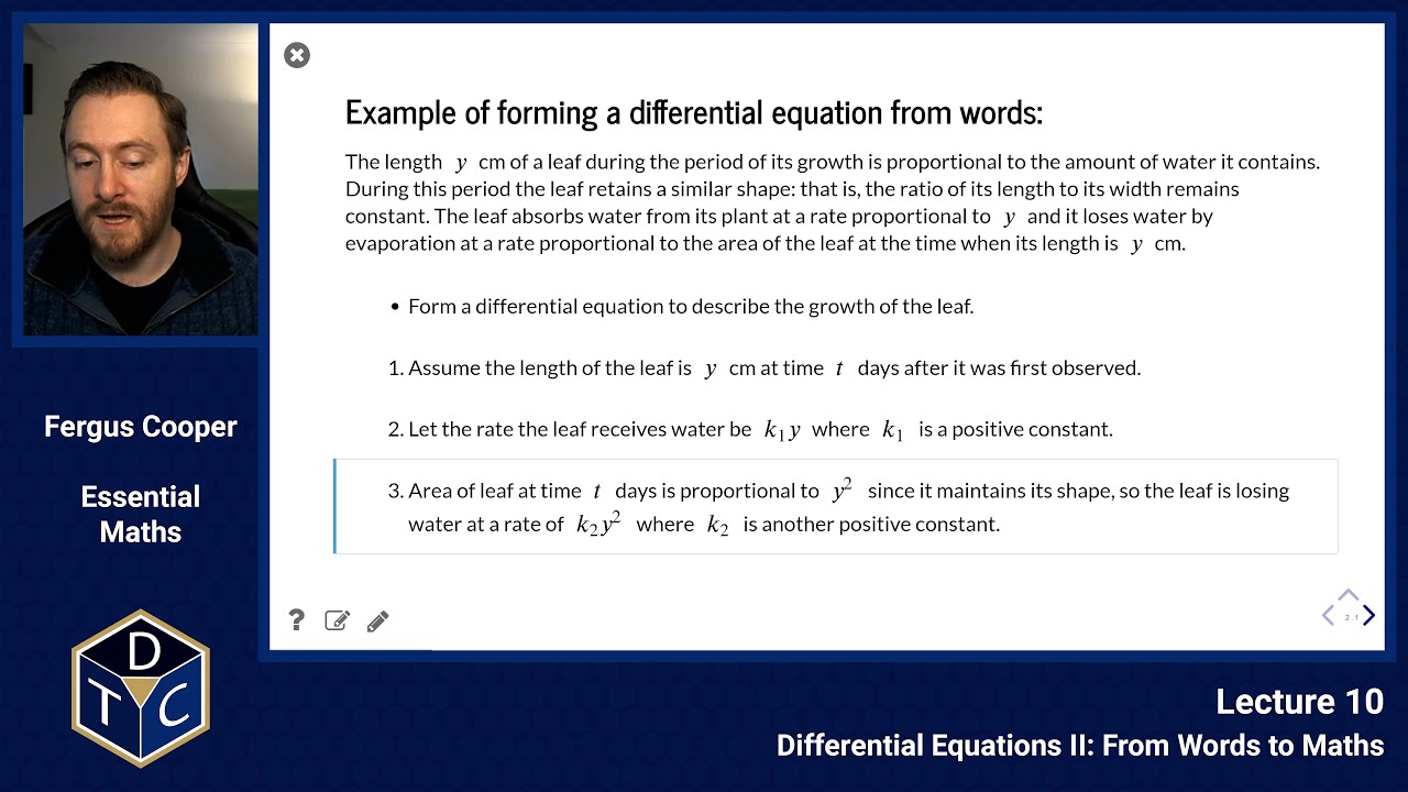
The length $y$ cm of a leaf during the period of its growth is proportional to the amount of water it contains. During this period the leaf retains a similar shape: that is, the ratio of its length to its width remains constant. The leaf absorbs water from its plant at a rate proportional to $y$ and it loses water by evaporation at a rate proportional to the area of the leaf at the time when its length is $y$ cm.

Assume the length of the leaf is $y$ cm at time $t$ days after it was first observed.
Let the rate the leaf receives water be $k_1y$ where $k_1$ is a positive constant.
Area of leaf at time $t$ days is proportional to $y^2$ since it maintains its shape, so the leaf is losing water at a rate of $k_2y^2$ where $k_2$ is another positive constant.
The length is proportional to the amount of water, so the rate of growth, $dy/dt$ , is proportional to the rate at which the leaf gains water, less the rate at which it loses it.

This gives us the equation:

\frac{dy}{dt}=k_1y-k_2y^2=y(k_1-k_2y)

We will solve it once we have looked at a second example.

Example 2: solid tumour growth

An avascular tumour tends to grow in a spherical shape, depending on environmental restrictions.

Assuming that the growth rate of the tumour depends only on the availability of oxygen and nutrients, which enter the tumour solely by diffusing through its surface, derive a model for the change in tumour volume over time.

Denote the volume of the tumour at time $t$ by $V(t)$ , and its radius by $R(t)$ .
Since the tumour is a sphere, its volume $V$ is proportional to $R^3$ and its surface area to $R^2$ , so the surface area is proportional to $V^{2/3}$ .
The rate at which the tumour acquires nutrients, and hence the rate at which the volume increases, is thus proportional to $V^{2/3}$ .

This gives us the equation:

\frac{dV}{dt} = kV^{2/3}

Solve by separation of variables:

\begin{aligned} \int V^{-2/3}\,dV &= \int k\,dt \\ 3V^{1/3} &= kt + c \\ V &= \left(\frac{kt+c}{3}\right)^3 \end{aligned}

where

c

is a constant of integration, the value of which will depend upon the initial conditions. If the volume at

t=0

V_0

, then

c = 3V_0^{1/3}

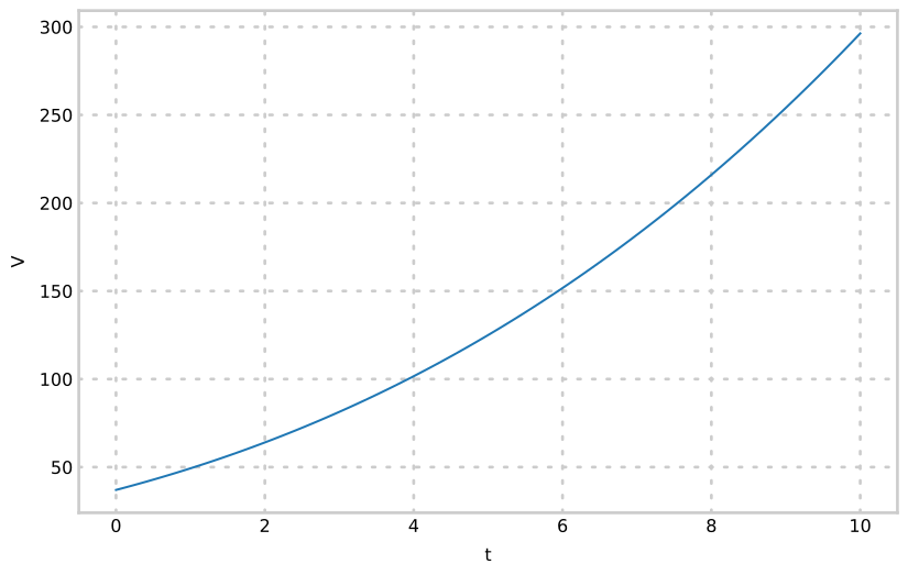
When

k=1

and

V_0=10

, the solution looks like the solid line below. For comparison, the dashed line shows exponential growth,

dV/dt = rV

, from the same volume and at the same initial rate (

r = kV_0^{-1/3}

). Because the nutrients enter only through the surface, the tumour falls further and further behind: its volume grows like

t^3

, and its radius, which is proportional to

V^{1/3} = V_0^{1/3} + kt/3

, grows at a constant rate.

Solution when k=1 and V0=10, against exponential growth from the same volume at the same initial rate

Example 1 again: solving the leaf equation

Let us return to, and solve, our leaf example:

\frac{dy}{dt}=k_1y-k_2y^2=y(k_1-k_2y)

This is a separable differential equation:

\int \frac{dy}{y(k_1-k_2y)} =\int dt.

To integrate the left-hand side, we split it into partial fractions, as in lecture 7. We want

\frac{1}{y(k_1-k_2y)}=\frac{A}{y}+\frac{B}{k_1-k_2y}.

Multiply both sides by

y(k_1-k_2y)

to get:

A(k_1-k_2y)+By=1 \qquad\text{so}\qquad Ak_1 + (B - Ak_2)y = 1

Equate the constant terms (coefficients of

y^0

Ak_1 = 1 \qquad\text{so}\qquad A=\frac{1}{k_1}

Equate coefficients of

y

B - Ak_2 = 0 \qquad\text{so}\qquad B=\frac{k_2}{k_1}

We can check this with SymPy's apart function:

import sympy as sp

y, k1, k2 = sp.symbols('y k_1 k_2')
sp.apart(1 / (y*(k1 - k2*y)), y)

- \frac{k_{2}}{k_{1} \left(- k_{1} + k_{2} y\right)} + \frac{1}{k_{1} y}

which agrees:

A=1/k_1

and

B=k_2/k_1

. Thus

\int \frac{dy}{k_1y}+\int \frac{k_2}{k_1(k_1-k_2y)}\,dy =\int dt.

While the leaf is growing,

0 < y < k_1/k_2

, so both logarithms are of positive numbers:

\frac{1}{k_1}\ln y-\frac{1}{k_1}\ln(k_1-k_2y)=t + c

To make

y

the subject, multiply by

k_1

and combine the logarithms, writing

d = k_1c

\ln\left(\frac{y}{k_1-k_2y}\right)=k_1t + d

Take the exponential of both sides, and multiply by

k_1-k_2y

y = (k_1-k_2y)e^{k_1t+d} \qquad\text{so}\qquad y\left(1 + k_2e^{k_1t+d}\right) = k_1e^{k_1t+d}

which gives

y=\frac{k_1 e^{k_1t+d}}{1+ k_2 e^{k_1t + d}}.

We can get

d

from the initial condition: if

y = y_0

t = 0

, then

e^d = y_0/(k_1-k_2y_0)

This is the logistic equation from lecture 3 (with

k = k_1

and

b = k_2

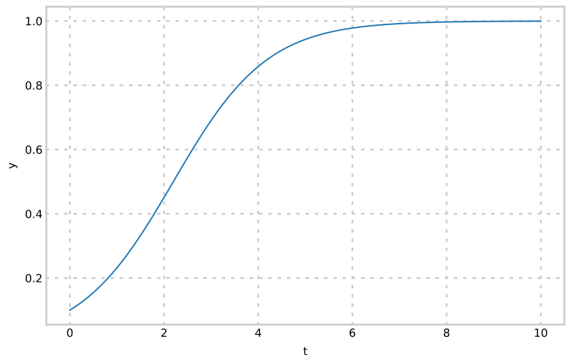
), and we will meet it again in lecture 11. As

t

grows,

y

levels off at

k_1/k_2

We can check our solution numerically, as in lecture 9:

import numpy as np
from scipy.integrate import solve_ivp

k1 = 1.0
k2 = 0.5
y0 = 0.1
t = np.linspace(0, 10, 100)
d = np.log(y0 / (k1 - k2*y0))
y_exact = (k1*np.exp(k1*t + d)
           / (1 + k2*np.exp(k1*t + d)))


def dydt(t, y):
    return k1*y - k2*y**2


solution = solve_ivp(dydt, [0, 10], [y0],
                     t_eval=t)
y_numerical = solution.y[0]

When

k_1 = 1

and

k_2 = 0.5

, the solution looks like:

Plot of the numerical vs exact solution of the leaf equation, when k1 = 1 and k2 = 0.5

The two lines lie on top of each other, and the leaf levels off at

k_1/k_2 = 2

Second order differential equations

The order of a differential equation is the order of the highest derivative in it.

Example 3

Let us try to solve the following second order equation:

\frac{d^2y}{dx^2} = \left(\frac{dy}{dx}\right)^2

We will use the substitution

z = dy/dx

. This implies that

\frac{dz}{dx} = \frac{d^2y}{dx^2}.

Substituting into the original equation, to eliminate

y

, gives

\frac{dz}{dx} = z^2

This is a separable equation:

\int z^{-2}\,dz = \int dx \qquad\Rightarrow\qquad-\frac{1}{z} = x + A \qquad\Rightarrow\qquad z = -\frac{1}{x+A}

where

A

is an arbitrary constant.

We can then replace

z

using the original substitution to obtain a first order differential equation:

\frac{dy}{dx} = -\frac{1}{x+A}

This equation can be solved with a standard integral:

y = -\ln(x+A) + B

How do we determine

A

and

B

? There are two constants, so we need two pieces of information. Determining the values of

A

and

B

can be done in several different ways, depending on the kind of information we have.

Case 1

Maybe we know that at

x=0

dy/dx = -1

and

y=0

Substitute the first condition into

dy/dx = -1/(x+A)

-1 = -\frac{1}{0+A} \qquad\text{so}\qquad A=1

Then substitute

A=1

and the second condition into

y = -\ln(x+A) + B

0 = -\ln 1 + B \qquad\text{so}\qquad B=0

So the solution is

y = -\ln(x+1)

Case 2

Maybe instead we know that

y(0)=0

and

y(e-1)=-1

: two values of

y

, and no value of

dy/dx

This time both conditions go into the solution

y = -\ln(x+A) + B

. The first,

y(0)=0

, gives:

0 = -\ln A + B \qquad\text{so}\qquad B=\ln A

Then substitute

B = \ln A

and the second condition,

y(e-1)=-1

-1 = -\ln(e-1+A) + \ln A = \ln\left(\frac{A}{e-1+A}\right)

Take the exponential of both sides, and solve for

A

\begin{aligned} e^{-1} &= \frac{A}{e-1+A} \\ e-1+A &= eA \\ e-1 &= (e-1)A \\ A &= 1 \end{aligned}

B = \ln 1 = 0

, and

y = -\ln(x+1)

: the same solution as in case 1.

Introductory problems

For more practice, an AI tool can write new problems like the ones below. Ask it for problems of the same type and difficulty, or for problems set in your own field. For example, you could ask it to "write five medicine problems on forming differential equations from words, at the level of these ones". Work them on paper first, then ask the tool to check your answers and to explain any step you are unsure of.

Introductory problems 1

Find the general solutions of the following differential equations:

$dy/dx = x^2 + e^x$
$dy/dx = y^2/x$
$(1/x)\,dy/dx = e^{4x}$
$dy/dx = -2xy$

Check your answers by differentiating them.

In each case,

C

and

A

are arbitrary constants.

Integrate both sides:
$y = \int\left(x^2 + e^x\right)dx = \frac{x^3}{3} + e^x + C$
Separate the variables:
$\int\frac{dy}{y^2} = \int\frac{dx}{x} \quad\Rightarrow\quad -\frac{1}{y} = \ln|x| + C \quad\Rightarrow\quad y = -\frac{1}{\ln|x| + C}$
(Dividing by $y^2$ assumes $y \neq 0$ : $y = 0$ is also a solution.)
Multiply both sides by $x$ and integrate, using integration by parts with $u = x$ and $v' = e^{4x}$ :
$y = \int xe^{4x}\,dx = \frac{xe^{4x}}{4} - \int\frac{e^{4x}}{4}\,dx = \frac{xe^{4x}}{4} - \frac{e^{4x}}{16} + C$
Separate the variables:
$\int\frac{dy}{y} = -\int 2x\,dx \quad\Rightarrow\quad \ln|y| = -x^2 + C \quad\Rightarrow\quad y = Ae^{-x^2}$

Introductory problems 2

Write down a differential equation for each of the following, defining any symbols and constants you use, and saying whether each constant is positive or negative. Do not solve them.

A drug is cleared from the blood at a rate proportional to the amount of drug present.
A population of cells grows at a rate proportional to its size, and cells are also removed (harvested) at a constant rate.
A spherical raindrop evaporates at a rate proportional to its surface area. Write an equation for its volume, and then one for its radius.
A rumour spreads through a group of fixed size at a rate proportional to both the number of people who have heard it and the number who have not.

Let $D$ be the amount of drug in the blood at time $t$ . The amount is decreasing, so
$\frac{dD}{dt} = -kD$
where $k$ is a positive constant.
Let $N$ be the number of cells at time $t$ . Growth adds cells at a rate $rN$ and harvesting removes them at a rate $h$ , so
$\frac{dN}{dt} = rN - h$
where $r$ and $h$ are positive constants.
Let $V$ be the volume of the raindrop and $r$ its radius at time $t$ . Its surface area is $4\pi r^2$ , and the volume is decreasing, so
$\frac{dV}{dt} = -k\,4\pi r^2$
where $k$ is a positive constant. Since $V = \frac{4}{3}\pi r^3$ , the chain rule gives
$\frac{dV}{dt} = 4\pi r^2\frac{dr}{dt}$
Setting the two expressions for $dV/dt$ equal and dividing by $4\pi r^2$ gives
$\frac{dr}{dt} = -k$
So, the radius of the raindrop shrinks at a constant rate.
Let the group contain $M$ people, and let $y$ be the number who have heard the rumour at time $t$ . Then $M - y$ people have not heard it, so
$\frac{dy}{dt} = ky(M - y)$
where $k$ is a positive constant. This has the same form as the leaf equation, $dy/dt = y(k_1 - k_2y)$ , from the lecture.

Introductory problems 3

Split each of the following into partial fractions by hand, and check your answers using sp.apart. Then integrate each one with respect to

x

$\frac{1}{x(x+1)}$
$\frac{x+5}{(x-1)(x+2)}$

Use your answer to part 1. to find the general solution of the differential equation

dy/dt = y(y+1)

We want
$\frac{1}{x(x+1)} = \frac{A}{x} + \frac{B}{x+1}$
Multiplying both sides by $x(x+1)$ gives $1 = A(x+1) + Bx$ . Setting $x = 0$ gives $A = 1$ , and setting $x = -1$ gives $B = -1$ . So,
$\int\frac{dx}{x(x+1)} = \int\left(\frac{1}{x} - \frac{1}{x+1}\right)dx = \ln|x| - \ln|x+1| + C$
We want
$\frac{x+5}{(x-1)(x+2)} = \frac{A}{x-1} + \frac{B}{x+2}$
Multiplying both sides by $(x-1)(x+2)$ gives $x + 5 = A(x+2) + B(x-1)$ . Setting $x = 1$ gives $6 = 3A$ , so $A = 2$ , and setting $x = -2$ gives $3 = -3B$ , so $B = -1$ . So,
$\begin{aligned} \int\frac{x+5}{(x-1)(x+2)}\,dx &= \int\left(\frac{2}{x-1} - \frac{1}{x+2}\right)dx \\ &= 2\ln|x-1| - \ln|x+2| + C \end{aligned}$

In Python:

import sympy as sp

x = sp.symbols('x')
print(sp.apart(1 / (x*(x + 1)), x))
print(sp.apart((x + 5) / ((x - 1)*(x + 2)), x))

-1/(x + 1) + 1/x
-1/(x + 2) + 2/(x - 1)

For the differential equation, separate the variables and use part 1.:

\int\frac{dy}{y(y+1)} = \int dt \qquad\Rightarrow\qquad \ln\left|\frac{y}{y+1}\right| = t + C

Taking the exponential of both sides gives

y/(y+1) = Ae^t

, where

A

is an arbitrary constant. Then

y = Ae^t(y+1)

, so

y(1 - Ae^t) = Ae^t

and

y = \frac{Ae^t}{1 - Ae^t}

(Dividing by

y(y+1)

assumes

y \neq 0

and

y \neq -1

. The solution

y = 0

is the case

A = 0

, and

y = -1

is also a solution.)

Main problems

Main problems 1

A circular patch of oil on the surface of some water has a radius

r

metres at time

t

minutes. When

t=0

minutes,

r=1\,

m and when

t=10

minutes,

r=2\,

Predict the value $T$ of $t$ when $r=4\,$ m, using a simple model in which the rate of increase of $r$ is taken to be constant. Find $T$ for this model.
In a more refined model, the rate of increase of $r$ is taken to be proportional to $1/r$ . Express this statement as a differential equation, and find the general solution. Find $T$ for this model.
Compare the two models used in 1. and 2., by sketching $r(t)$ on the same figure or plotting using Python. Comment on the differences seen during different time intervals.

If $dr/dt$ is a constant $a$ , then $r = at + C$ . $r(0) = 1$ gives $C = 1$ , and $r(10) = 2$ gives $a = 0.1$ , so $r = 1 + 0.1t$ . Then $r = 4$ when $4 = 1 + 0.1T$ , so $T = 30$ minutes.
The rate of increase is proportional to $1/r$ :
$\frac{dr}{dt} = \frac{k}{r}$
where $k$ is a positive constant. Separate the variables:
$\int r\,dr = \int k\,dt \quad\Rightarrow\quad \frac{r^2}{2} = kt + C$
so the general solution is $r = \sqrt{2kt + 2C}$ . $r(0) = 1$ gives $C = 1/2$ , and $r(10) = 2$ gives $2 = 10k + 1/2$ , so $k = 3/20$ . So, $r^2 = 1 + 0.3t$ . Then $r = 4$ when $16 = 1 + 0.3T$ , so $T = 50$ minutes.

Both models agree at

t = 0

and

t = 10

import numpy as np
from matplotlib import pyplot as plt

t = np.linspace(0, 60, 200)

plt.plot(t, 1 + 0.1 * t, label='constant rate')
plt.plot(t, np.sqrt(1 + 0.3 * t), label='rate proportional to 1/r')
plt.xlabel('t (minutes)')
plt.ylabel('r (m)')
plt.legend()

Between

t = 0

and

t = 10

, the second model grows faster, as its rate is largest when

r

is small. After

t = 10

, it grows more and more slowly, and falls behind the constant-rate model, which is why it takes longer to reach 4m.

Main problems 2

A nuclear installation local to Oxford 'lost' 17g of Cobalt-60 between two inspections 6 months apart. A spokesperson told a newspaper reporter that the loss was due to 'natural radioactive decay' during that period.

If this explanation was correct, what mass of Cobalt was stored on the site? (The half life of

^{60}

Co =

5.26

years.)

Let

M

be the mass of Cobalt-60 at the first inspection. Radioactive decay gives

m = Me^{-\lambda t}

, with

\lambda = \frac{\ln 2}{t_{1/2}} = \frac{\ln 2}{5.26} \approx 0.132\,\text{year}^{-1}

After 6 months,

t = 0.5

years, and the mass lost is

M - Me^{-0.5\lambda} = M\left(1 - e^{-0.5\lambda}\right) = 17

So,

M = \frac{17}{1 - e^{-0.5\lambda}} \approx \frac{17}{0.0638} \approx 267\,\text{g}

If the explanation was correct, about 267g of Cobalt-60 was stored on the site.

Main problems 3

By making a substitution

z = dy/dx

, solve the equation

\frac{d^2y}{dx^2} = (1-3x^2)\left(\frac{dy}{dx}\right)^2\quad\text{with}\quad y(2) = 0\quad\text{and}\quad y'(2) = 1/6.

Hint: you will need to use partial fractions for part of this question, to break up

\frac{1}{x^3-x} = \frac{-1}{x} + \frac{1/2}{x+1} + \frac{1/2}{x-1}.

With

z = dy/dx

, we have

d^2y/dx^2 = dz/dx

, so the equation becomes a first order equation for

z

\frac{dz}{dx} = (1-3x^2)z^2

Separate the variables:

\int\frac{dz}{z^2} = \int(1-3x^2)\,dx \quad\Rightarrow\quad -\frac{1}{z} = x - x^3 + C

y'(2) = 1/6

means

z = 1/6

x = 2

, so

-6 = 2 - 8 + C

, and

C = 0

. So,

\frac{dy}{dx} = z = -\frac{1}{x - x^3} = \frac{1}{x^3 - x}

Now integrate, using the partial fractions in the hint:

\begin{aligned} y &= \int\left(-\frac{1}{x} + \frac{1/2}{x+1} + \frac{1/2}{x-1}\right)dx \\ &= -\ln|x| + \frac{1}{2}\ln|x+1| + \frac{1}{2}\ln|x-1| + D \end{aligned}

y(2) = 0

gives

0 = -\ln 2 + \frac{1}{2}\ln 3 + 0 + D

, so

D = \ln 2 - \frac{1}{2}\ln 3

. Combining the logs (for

x > 1

, near the starting point

x = 2

y = \frac{1}{2}\ln\left(x^2 - 1\right) - \ln x + \ln 2 - \frac{1}{2}\ln 3 = \frac{1}{2}\ln\left(\frac{4\left(x^2-1\right)}{3x^2}\right)

Main problems 4

Suppose a cell contains a chemical (the solute) dissolved in it at a concentration of

c(t)

, and the concentration of the same substance outside the cell is a constant

k

. By Fick's law, if

c(t)

and

k

are unequal, solute moves across the cell wall at a rate proportional to the difference between

c(t)

and

k

, towards the region of lower concentration.

Write down a differential equation which is satisfied by $c(t)$ .
Solve this differential equation with the initial condition $c(0)=c_0$ .
Sketch the solutions for $c_0 > k$ and $k > c_0$ .
Blood glucose concentration is 5.1 mM and the concentration inside the cell is at 0.1 mM. If glucose utilisation within the cell is totally inhibited, it takes 1 min for the intracellular concentration to reach 2.6 mM. How long would it take for the concentration to reach 5.0 mM?
Calculate the amount of glucose (moles) entering the cell to bring the concentration from 0.1 mM to 5 mM assuming the cell is spherical with a diameter of $10\,\mu$ m.

The rate of change of $c$ is proportional to the difference $k - c$ , and solute moves towards the lower concentration:
$\frac{dc}{dt} = \alpha(k - c)$
where $\alpha$ is a positive constant. If $c < k$ , then $dc/dt > 0$ and solute moves into the cell; if $c > k$ , it moves out.
Separate the variables:
$\int\frac{dc}{k - c} = \int\alpha\,dt \quad\Rightarrow\quad -\ln|k - c| = \alpha t + D \quad\Rightarrow\quad k - c = Be^{-\alpha t}$
$c(0) = c_0$ gives $B = k - c_0$ , so
$c = k - (k - c_0)\,e^{-\alpha t}$

In both cases

c

starts at

c_0

and approaches

k

exponentially. If

c_0 > k

c

decreases towards

k

; if

c_0 < k

c

increases towards

k

import numpy as np
from matplotlib import pyplot as plt

k = 1
t = np.linspace(0, 5, 200)

for c0 in [2, 0]:
    plt.plot(t, k - (k - c0) * np.exp(-t), label=f'c0 = {c0}')
plt.axhline(k, linestyle='--', color='grey')
plt.xlabel('t')
plt.ylabel('c')
plt.legend()

Here $k = 5.1$ and $c_0 = 0.1$ , so $c = 5.1 - 5e^{-\alpha t}$ . At $t = 1$ minute, $c = 2.6$ :
$2.6 = 5.1 - 5e^{-\alpha} \quad\Rightarrow\quad e^{-\alpha} = 0.5 \quad\Rightarrow\quad \alpha = \ln 2\,\text{min}^{-1}$
The concentration reaches 5.0mM when
$5.0 = 5.1 - 5e^{-\alpha t} \quad\Rightarrow\quad e^{-\alpha t} = \frac{1}{50} \quad\Rightarrow\quad t = \frac{\ln 50}{\ln 2} \approx 5.6\,\text{minutes}$
The volume of the cell, with radius $5\,\mu\text{m} = 5\times 10^{-6}\,$ m, is
$V = \frac{4}{3}\pi\left(5\times 10^{-6}\right)^3 \approx 5.24\times 10^{-16}\,\text{m}^3 = 5.24\times 10^{-13}\,\text{l}$
The concentration rises by $5.0 - 0.1 = 4.9\,\text{mM} = 4.9\times 10^{-3}\,\text{mol/l}$ , so the amount of glucose entering the cell is
$4.9\times 10^{-3} \times 5.24\times 10^{-13} \approx 2.57\times 10^{-15}\,\text{mol}$

Extension problems

Extension problems 1

Consider a simple model of the production and degradation of a protein. The protein is produced at a constant rate

k_1

, and degraded at a rate proportional to its concentration, with constant

k_2

Form and solve a differential equation describing the change in protein concentration.
What concentration is reached after 'sufficient' time has elapsed?

Let $s$ be the protein concentration at time $t$ , with $s(0) = s_0$ . It increases at rate $k_1$ and decreases at rate $k_2s$ , so
$\frac{ds}{dt} = k_1 - k_2s$
Separate the variables:
$\begin{aligned} &\int\frac{ds}{k_1 - k_2s} = \int dt \\ \quad\Rightarrow\quad &-\frac{1}{k_2}\ln|k_1 - k_2s| = t + C \\ \quad\Rightarrow\quad &k_1 - k_2s = Be^{-k_2t} \end{aligned}$
$s(0) = s_0$ gives $B = k_1 - k_2s_0$ , so
$s = \frac{k_1}{k_2} + \left(s_0 - \frac{k_1}{k_2}\right)e^{-k_2t}$
As $t\to\infty$ , $e^{-k_2t}\to 0$ , so $s \to k_1/k_2$ , whatever the starting concentration. At this concentration, production and degradation balance, and $ds/dt = 0$ .