This material has been adapted from material by Fergus Cooper and others from the "Essential Mathematics" module at the Doctoral Training Centre, University of Oxford.
This course material was developed as part of UNIVERSE-HPC, which is funded through the SPF ExCALIBUR programme under grant number EP/W035731/1
Differential equations 1
Learning outcomes
Understand the concept of a differential equation
Be able to use integration to solve simple differential equations
Be able to use the method of separation of variables to solve differential equations
Be able to use initial conditions to find the constants in a general solution
Be able to solve differential equations numerically, with Euler's method and with SciPy
YouTube lecture recording from October 2020
A recording of this lecture from October 2020; the material has changed a little since.
Why differential equations?
Many models in biology say how quickly something changes (e.g. a colony grows at a rate proportional to its size, or a radioactive sample decays at a rate proportional to the amount left).
Such a model is a differential equation, and solving it tells us how the quantity itself changes over time.
In this lecture we solve the simplest differential equations by integration, using the methods from the lectures on integration.
We also see how to solve them numerically with Python, which lets us check our solutions, and which works even when we cannot solve an equation by hand.
What is a differential equation?
If y is a variable that depends on the variable x, then a differential equation in x and y is one that relates dy/dx to x, to y, or to both.
We write
dxdy=f(x,y).
Solving a differential equation
The simplest differential equations are very similar to integration.
dxdy=x3+5x2+1
Put all the terms in y (just the derivative in this case) on the left, and all the terms involving x on the right.
dy=(x3+5x2+1)dx
Then we integrate both sides
∫dy=∫(x3+5x2+1)dx
The general solution to this equation is
y+A=∫(x3+5x2+1)dx=41x4+35x3+x+B
where A and B are arbitrary constants.
It is called the general solution because it holds for any values of the constants, so it describes a whole family of curves.
If we are given the initial conditions, say, y=0 when x=0 (often written as y(0)=0), we can determine the value for the constants.
In this example A=B.
Separation of variables
This approach can be generalised into what is known as the separation of variables method.
Separation of variables: example 1
dxdy=2x+c
The equation is already separated, with all terms in y (just the derivative in
this case) on the left, and terms involving x on the right.
Is this right?
We can check by solving the differential equation numerically, and comparing the result with our solution.
Solving numerically: Euler's method
The simplest way to solve a differential equation numerically is Euler's method.
At the start, x0, we know y0, and the differential equation gives us the gradient there, f(x0,y0).
Take a small step h along the tangent:
x1=x0+hy1=y0+hf(x0,y0)
Then repeat from the new point, and so on:
yn+1=yn+hf(xn,yn)
Each step follows the tangent, so the answer drifts away from the true solution where the curve bends.
So, the smaller the step, the more accurate the answer (but the more steps we need).
Here is Euler's method in Python, for example 1 with c=1.
We start at x=1, where y(1)=c, and take 9 steps of size 1, to reach x=10:
c =1.0defdydx(x, y):return2*x + c
h =1.0# the step sizen =9# the number of steps, from x = 1 to x = 10x =1.0# start at x = 1,y = c # where y(1) = cfor step inrange(n): y = y + h * dydx(x, y)# a step along the tangent x = x + h
print(y)
100.0
At the end of the loop, y holds our estimate of y(10).
Running the code with smaller steps (and more of them) gives, to two decimal places:
Step size h
Number of steps n
y(10)
1
9
100.00
0.1
90
108.10
0.01
900
108.91
The exact value is y(10)=102+10−1=109, so a step 10 times smaller makes the error about 10 times smaller.
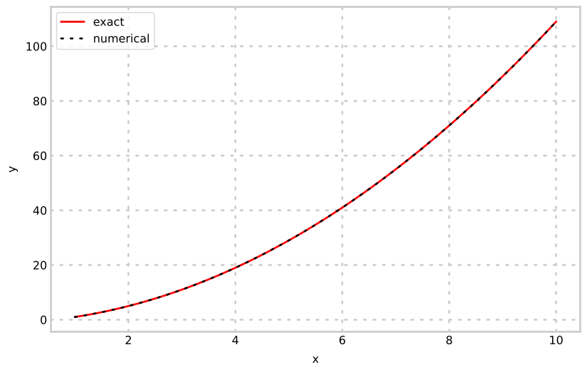
Here is the solution with h=1, against the exact solution:
The curve bends upwards, so each step along the tangent falls a little below it, and the errors add up.
Solving numerically in practice
Euler's method needs very small steps to be accurate.
In practice we use more sophisticated methods, such as SciPy's solve_ivp, which take better steps and choose the step size for us.
solve_ivp takes a function of the independent variable and y (in that order), the interval, and the initial value.
It returns the solution at the points we ask for with t_eval.
Here we use it to check example 1:
import numpy as np
from scipy.integrate import solve_ivp
c =1.0A =-1.0x0 =1.0x1 =10.0x = np.linspace(x0, x1,100)y_exact = x**2+ c*x + A
defdydx(x, y):return2*x + c
solution = solve_ivp(dydx,[x0, x1],[c], t_eval=x)y_numerical = solution.y[0]
The two lines lie on top of each other, so our solution, with A=−1, is right.
Separation of variables: example 2
dxdy=5x23y
Separate the variables so that all the terms in x are on one side of the equation and all the terms in y are on the other side:
y1dxdy=5x23
Integrating both sides with respect to x:
∫y1dxdydx=∫5x23dx⇒∫y1dy=∫5x23dx
Why we can separate the variables
It can look as though we are splitting dy/dx up like a fraction, which seems suspicious.
In fact the chain rule makes this work.
Suppose dy/dx=f(x)g(y).
Divide by g(y), and integrate both sides with respect to x:
∫g(y)1dxdydx=∫f(x)dx
If H is an antiderivative of 1/g, so that H′(y)=1/g(y), then by the chain rule
dxdH(y)=H′(y)dxdy=g(y)1dxdy
So the left-hand side is just H(y)+C, i.e. the integral of 1/g(y) with respect to y (this is integration by substitution, from the lecture on integration):
∫g(y)1dy=∫f(x)dx
This means that we can treat dy/dx as if it were a fraction, and the chain rule makes sure we get the right answer.
There is one thing to watch.
Dividing by g(y) only works where g(y) is not zero, so a constant solution with g(y)=0 can be lost.
In this example g(y)=y, and y=0 is also a solution, as we see below.
Now integrate on each side:
ln∣y∣+A=5/25x25+B=2x25+B
So:
ln∣y∣=2x25+CwhereC=B−A
Taking the exponential of both sides gives ∣y∣=eCe2x5/2, so
y=De2x25whereD=±eC
The constant D can be positive or negative, depending on the sign of y.
It can also be zero, which gives the solution y=0 that we lost when we divided by y.
Substituting the initial condition y(0)=0 gives 0=−2+c3, so c3=2 and
y=±2−2e−x(1+x)
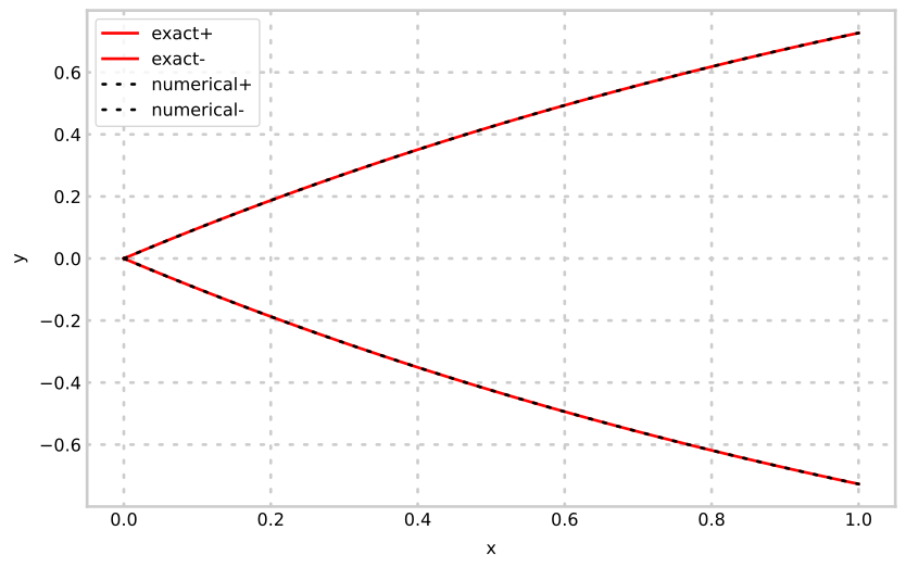
We check this numerically, as before:
c3 =2.0x0 =0.0x1 =1.0x = np.linspace(x0, x1,100)# the positive solutiony_exact = np.sqrt(-2*np.exp(-x)*(1+ x)+ c3)defdydx(x, y):return np.exp(-x)* x / y
solution = solve_ivp(dydx,[x0, x1],[1e-8], t_eval=x, rtol=1e-8)y_numerical = solution.y[0]
Notice that we start from y=10−8 rather than zero.
The function dydx divides by y, so it cannot be evaluated at y=0, and solve_ivp cannot take its first step.
Starting just above zero avoids this, and changes the solution very little.
The argument rtol asks for a more accurate solution than the default.
Here we have checked the positive solution.
The negative solution is its mirror image, and we would find it by starting just below zero.
Application: bacterial growth
Suppose the growth rate of a bacterial colony is proportional to its size, and that we observe that the colony triples in size after 10 hours.
How long will it take to reach 11 times its original size?
Let N represent the number of bacteria, and suppose there are N0 at time t=0.
We are given that when t=10 hours, N=3N0, and need to find the time at which N=11N0.
The equation of growth is:
dtdN=kN
where k is a positive constant.
We can solve this by separation of variables, to obtain lnN=kt+c (we can write lnN rather than ln∣N∣, as N is positive).
Using the t=0 condition, we have that lnN0=c, so
lnN0N=kt
We can use the data from t=10 to find k:
lnN03N0=10k⇒k=10ln3≈0.11hr−1
To find t when N=11N0:
lnN011N0=kt⇒t=kln11=ln310ln11≈21.8 hours
Notice that we used the exact value of k here, rather than the rounded 0.11, so that the rounding does not affect the answer.
Application: radioactive decay
The rate at which a sample decays is proportional to the amount left, i.e.
dtdN=−λN
where N is the mass of radioactive atoms at time t and λ is called the decay constant.
The element radium (atomic mass 226) has a decay constant of 13.6×10⁻¹²s−1.
Solving the differential equation via separation of variables, we obtain the general solution
N=Be−λt(1)
Consider an arbitrary initial condition: at t=t0, N=N0.
Then:
N0=Be−λt0⇒B=N0eλt0
Substituting in (1) gives the solution
N=N0e−λ(t−t0)(2)
The half-life, t1/2, is the time taken for N to reduce by half.
(The last line uses ln(1/2)=−ln2.)
Note that this time is independent of the initial value N0.
The half-life for radium is thus
t1/2=13.6×10−12ln2≈5.10×1010s,
or about 1600 years.
Order of a reaction
The power to which the concentration of a species is raised in a rate law is the order of the process/reaction with respect to that species.
A reaction with the rate law
dtdX=k2[A][B]
is first order in A and first order in B.
The overall order of a process/reaction is the sum of the orders of all the components.
This rate law is thus second order overall.
Note that this is different from the order of a differential equation, which is given by the highest derivative.
Both zeroth and first order processes are modelled below by first order differential equations.
Zeroth order processes
The rate of change is independent of concentration, i.e. the rate of change is proportional to concentration raised to power zero.
dtdAdtdA=k(growth)=−k(decay)
General solutions:
AA=A0+k(t−t0)=A0−k(t−t0)
The concentration rises or falls in a straight line.
First order processes
The rate of change depends on the concentration of one species, i.e. the rate of change is proportional to concentration raised to first power.
dtdAdtdA=kA(growth)=−kA(decay)
General solutions:
AA=A0ek(t−t0)=A0e−k(t−t0)
For decay, the half-life is a constant, i.e. it is independent of the amount there at the beginning, as we found for radioactive decay.
When k=2.0 the two different solutions look like this:
Application: enzyme kinetics
In lecture 1 we met the Michaelis-Menten equation for the rate of an enzyme reaction.
The rate is how quickly the substrate is used up, so
dtds=−Km+sVmaxs
where s=[S] is the substrate concentration, and Vmax and Km are constants.
By integration, we will derive expressions relating substrate concentration to time
when s≫Km
when s≪Km
and sketch the graphs of s against t in each case.
Large concentrations
When s≫Km, Km in the differential equation's denominator can be neglected:
dtds≈−sVmaxs=−Vmax
The rate of change in concentration is a constant, so this is a zeroth order process.
We can integrate directly to obtain
s=∫−Vmaxdt=−Vmaxt+c
where c is a constant of integration.
If s(0)=s0, then c=s0.
The graph thus has slope −Vmax and crosses the vertical axis at s=s0.
Small concentrations
When s≪Km, s in the differential equation's denominator can be neglected:
dtds≈−KmVmaxs
The rate of change in concentration depends on the concentration, so this is a first order process.
∫s1dslnss=−∫KmVmaxdt=−KmVmaxt+Dwhere D is a constant=Be−Vmaxt/Kmwhere B=eD
(We can write lns rather than ln∣s∣, as a concentration is positive.)
On a graph s crosses the vertical axis at s=B and decreases with time exponentially.
Solving numerically
Let's look at this numerically using the original equation, with Vmax=1 and s(0)=1:
dtds=−Km+sVmaxs
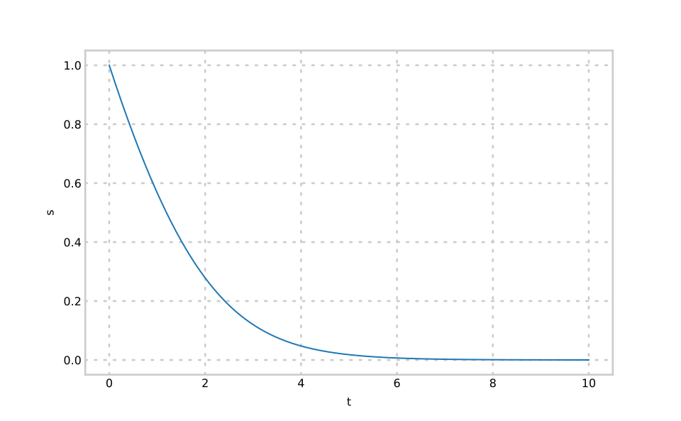
When Km=0.2, s starts much larger than Km, and falls in a nearly straight line, like a zeroth order process.
As s becomes small, it levels off exponentially, like a first order process:
When Km=1.0, s is never much larger than Km, and the decline looks more like a first order process throughout:
Introductory problems
For more practice, an AI tool can write new problems like the ones below.
Ask it for problems of the same type and difficulty, or for problems set in your own field.
For example, you could ask it to "write five microbiology problems on separable differential equations, at the level of these ones".
Work them on paper first, then ask the tool to check your answers and to explain any step you are unsure of.
Introductory problems 1
Find the general solutions of the following differential equations:
dy/dx=x
dr/dt=−sin(πt)
dy/dx=bx2
(x−4)dy/dx=3y
udu/dv=v+6
7exdy/dx=x/y
Check your answers by differentiating them.
In each case, C, A and D are arbitrary constants.
Integrate both sides with respect to x:
y=∫xdx=2x2+C
r=−∫sin(πt)dt=πcos(πt)+C
y=∫bx2dx=3bx3+C
Separate the variables:
∫ydy=∫x−43dx⇒ln∣y∣=3ln∣x−4∣+D
So, y=A(x−4)3, where A=±eD.
The variables are already separated:
∫udu=∫(v+6)dv⇒2u2=2v2+6v+D
So, u2=v2+12v+C, or u=±v2+12v+C.
Separate the variables, as in example 3 of the lecture:
∫7ydy=∫xe−xdx
Integrating the right-hand side by parts, with u=x and v′=e−x, gives −xe−x−e−x, so
27y2=−e−x(x+1)+D⇒y2=−72e−x(x+1)+C
Introductory problems 2
Find the solution to the following differential equations subject to the specified boundary conditions:
dy/dx=1/xwithy(2)=0
dy/dx=ywithy(0)=1
Use Python's scipy.integrate.solve_ivp to verify your solutions
# hintimport numpy as np
from scipy.integrate import solve_ivp
import matplotlib.pyplot as plt
# you need a function that calculates dy/dx# solve_ivp passes the independent variable (here x) first, then ydefdydx(x, y):return1/ x
y0 =0# <-- the y-value of the initial conditionx0 =2# <-- the x-value of the initial condition# the x-values at which to calculate the solutionx = np.linspace(x0, x0 +10,1000)# solve ODE numericallysolution = solve_ivp(dydx,[x[0], x[-1]],[y0], t_eval=x)y = solution.y[0]# plot the numerical solution and your hand-calculated# solution, and check that they agree
Separate the variables and integrate:
y=∫xdx=lnx+C
(We can write lnx rather than ln∣x∣, as the solution starts at x=2.)
y(2)=0 gives C=−ln2, so
y=lnx−ln2=ln2x
Separate the variables:
∫ydy=∫dx⇒lny=x+C⇒y=Aex
y(0)=1 gives A=1, so y=ex.
To check with Python, we compare the numerical solution with our solution.
Here we ask solve_ivp for more accuracy than the default, with rtol:
import numpy as np
from scipy.integrate import solve_ivp
import matplotlib.pyplot as plt
defdydx(x, y):return1/ x
x = np.linspace(2,12,1000)solution = solve_ivp(dydx,[x[0], x[-1]],[0], t_eval=x, rtol=1e-8)y_exact = np.log(x /2)print('largest difference =', np.max(np.abs(solution.y[0]- y_exact)))plt.plot(x, y_exact, label='exact')plt.plot(x, solution.y[0],'--', label='numerical')plt.xlabel('x')plt.ylabel('y')plt.legend()
largest difference = 2.4351254179766357e-06
For 2., ex grows quickly, so we look at the difference relative to the size of y:
defdydx(x, y):return y
x = np.linspace(0,5,1000)solution = solve_ivp(dydx,[x[0], x[-1]],[1], t_eval=x, rtol=1e-8)y_exact = np.exp(x)print('largest relative difference =', np.max(np.abs(solution.y[0]- y_exact)/ y_exact))
largest relative difference = 2.0386919889137807e-07
In both cases the numerical and exact solutions agree closely, and the two curves lie on top of each other.
Main problems
Main problems 1
The number of bacteria present in a given culture increases at a rate proportional to the number present.
When first observed, the culture contained n0 bacteria, and two hours later it contained n1.
Find the number present t hours after observations began.
How long did it take for the number of bacteria to triple?
Sketch a curve of the solution to the equation that you derive.
What assumptions are implicit in this model of bacterial growth?
Let n be the number of bacteria at time t hours.
The rate of increase is proportional to n, so
dtdn=kn
where k is a positive constant.
Separating the variables, as for bacterial growth in the lecture, gives n=n0ekt, since n=n0 at t=0.
At t=2, n=n1, so
n1=n0e2k⇒k=21lnn0n1
So, the number present after t hours is
n=n0e2tln(n1/n0)=n0(n0n1)t/2
The number has tripled when n=3n0, so ekt=3, and
t=kln3=ln(n1/n0)2ln3 hours
The curve starts at n=n0 when t=0 and grows exponentially, more and more steeply, passing through n1 at t=2:
import numpy as np
from matplotlib import pyplot as plt
n0 =1n1 =2# for examplet = np.linspace(0,10,200)plt.plot(t, n0 *(n1 / n0)**(t /2))plt.xlabel('t (hours)')plt.ylabel('n')
The model assumes that every bacterium divides at the same constant rate, whatever the size of the population.
This means there are unlimited nutrients and space, no bacteria die, and nothing else (such as temperature) changes.
In practice, growth slows as resources run out, so the model only describes the early stages of growth.
Main problems 2
Solve:
y2dy/dx=2x/3withy(2)=1
dy/dx=β/xwithy(1)=0. Find β such that y(e3)=1.
dy/dx=a0+a1x+a2x2+a3x3+a4x4withy(0)=π
Separate the variables:
∫y2dy=∫32xdx⇒3y3=3x2+C⇒y3=x2+3C
y(2)=1 gives 1=2+3C, so 3C=−1, and
y=(x2−1)1/3
Integrate both sides:
y=β∫xdx=βlnx+C
y(1)=0 gives C=0, so y=βlnx.
Then y(e3)=1 gives βln(e3)=3β=1, so β=1/3.
Integrate both sides term by term:
y=a0x+2a1x2+3a2x3+4a3x4+5a4x5+C
y(0)=π gives C=π, so
y=π+a0x+2a1x2+3a2x3+4a3x4+5a4x5
Main problems 3
In a certain chemical reaction, substance A is transformed into product P.
The mass of A at any given time, t, is mt, and the rate of transformation of A at time t is proportional to mt.
Given that the original mass of A is 130g, and that 50g has been transformed after 150 seconds:
Form and solve the differential equation relating mt to t.
Find the mass of A transformed over a 300s period.
Sketch a graph of mt versus t.
A is used up at a rate proportional to mt, so
dtdmt=−kmt
where k is a positive constant.
Separating the variables gives mt=130e−kt, since m0=130g.
After 150 seconds, 50g has been transformed, so m150=80g:
So, the mass transformed is 130−49.2≈80.8g.
(The first 150 seconds transforms 50g, but the next 150 seconds only about 30.8g, because there is less A left.)
mt starts at 130g and decays exponentially towards zero, falling quickly at first and then more and more slowly:
import numpy as np
from matplotlib import pyplot as plt
k = np.log(130/80)/150t = np.linspace(0,1500,200)plt.plot(t,130* np.exp(-k * t))plt.xlabel('t (s)')plt.ylabel('mass of A (g)')
Main problems 4
Newton's law of cooling states that the rate of decrease of the temperature of a body is proportional to the amount by which its temperature exceeds the temperature of its surroundings.
If T0 is the initial temperature of a body, Ts is the temperature of its surroundings, and T is the temperature of the body at time t:
Form a differential equation for Newton's Law of cooling.
Show that T−Ts=(T0−Ts)e−kt, where k is a constant, and state the units of the constant k.
Glycerol is to be added to a protein sample prior to storage.
The glycerol is heated to 65∘C to aid accurate pipetting.
To avoid denaturation of the sample, the glycerol must then be allowed to cool to below 29∘C before being added to the protein.
If the ambient temperature is 22∘C, the glycerol cools to T=59∘C at time t=2 minutes.
At what time can the glycerol be added to the protein?
Using a choice of axes that will allow you easily to predict the temperature of the glycerol, sketch a graph of the anticipated variation of the glycerol temperature with time.
Once the glycerol has been added to the protein, will the rate of cooling be described by the same constant k? Give reasons for your answer.
The rate of decrease of T is proportional to T−Ts, so
dtdT=−k(T−Ts)
where k is a positive constant.
Separate the variables (Ts is a constant):
∫T−TsdT=−∫kdt⇒ln(T−Ts)=−kt+C
At t=0, T=T0, so C=ln(T0−Ts), and
lnT0−TsT−Ts=−kt⇒T−Ts=(T0−Ts)e−kt
The exponent kt must have no units, so k has units of time−1, for example min−1.
Here T0=65, Ts=22 and T=59 at t=2 minutes:
59−22=(65−22)e−2k⇒k=21ln3743≈0.0751min−1
The glycerol reaches 29∘C when
29−22=43e−kt⇒t=k1ln743≈24.2minutes
So, the glycerol can be added after about 24 minutes.
Taking logs of the solution gives
ln(T−Ts)=ln(T0−Ts)−kt
So, plotting ln(T−22) against t gives a straight line, with intercept ln43 and gradient −k.
We can read off the time for any temperature, or extend the line, by using a ruler:
import numpy as np
from matplotlib import pyplot as plt
k = np.log(43/37)/2t = np.linspace(0,30,100)T =22+43* np.exp(-k * t)plt.plot(t, np.log(T -22))plt.xlabel('t (minutes)')plt.ylabel('ln(T - 22)')
No.
The constant k depends on the body that is cooling: its mass, heat capacity and surface area, and the container it is in.
Once the glycerol is mixed with the protein sample, it is a different body, so it will cool with a different constant.
Main problems 5
The amount of 14C (radioactive carbon-14) in a sample is measured using a Geiger counter, which records each disintegration of an atom.
The rate at which 14C decays is proportional to the amount present.
The half-life of 14C is about 5730 years.
This means that half of the sample will have disintegrated after 5730 years.
In living tissue, 14C disintegrates at a rate of about 13.5 atoms per minute per gram of carbon.
Because living tissue is constantly exchanging carbon with its environment, the proportion of 14C among its carbon atoms remains constant over time.
Once the tissue is no longer living, this constant exchange of carbon ceases and the fraction of 14C among its carbon atoms begins to get smaller.
Consequently, the disintegration rate drops.
In 1977 a charcoal fragment found at Stonehenge on the Salisbury Plain recorded 8.2 disintegrations per minute per gram of carbon: about 60% of that for living tissue.
Assuming that the charcoal was formed during the building of the site, use this information to estimate the date at which Stonehenge was built.
Let N be the amount of 14C in the charcoal, t years after it formed.
The rate of decay is proportional to N, so, as for radioactive decay in the lecture,
N=N0e−λtwithλ=t1/2ln2=5730ln2≈1.21×10−4year−1
The disintegration rate is λN, which is proportional to N, so it decays in the same way.
It started at 13.5 per minute per gram, and had fallen to 8.2 by 1977:
8.2=13.5e−λt⇒t=λ1ln8.213.5≈4120years
So, the charcoal formed about 4120 years before 1977, which is about 2145 BC.
In practice, the amount of 14C in the atmosphere has changed over time, so radiocarbon dates have to be calibrated against samples of known age, such as tree rings.
Calibrated dates put the building of Stonehenge at about 3000 BC.
Extension problems
Extension problems 1
The absorbanceA of a solution is given by the equation:
A=log10(IIo)
where Io is the intensity of the light impinging on the solution (incident light) and I is the intensity of the light emerging from it (transmitted light).
The Beer-Lambert law states that
A=ϵ⋅c⋅l
where ϵ is the molar absorption coefficient of the solute, c is the concentration of the solute and l is the distance that the light has travelled through the solution.
The transmittanceT is defined as the fraction of incident light transmitted through the solution (T=I/Io).
Derive an expression relating the transmittance, T, of the solution to ϵ, c and l.
The attenuationQ of the light beam is defined as the difference between the intensities of the incident and the transmitted light (Q=Io−I).
Derive an expression for the attenuation of the light beam when a beam of light intensity Io traverses a distance l through a solution of fixed concentration c.
Sketch a graph showing the dependence of Q on l in a solution of fixed concentration.
ATP has a molar absorption coefficient of 15.7×10³M−1cm−1.
Calculate the initial rate (in watts/cm) at which light intensity is attenuated when a light beam of intensity 200 watts enters a 10μM solution of ATP.
What would happen to this rate if
the concentration of ATP is doubled;
the intensity of the incident light is doubled;
the length of the cell holding the solution is doubled?
Since T=I/Io, the absorbance is A=log10(1/T)=−log10T.
The Beer-Lambert law then gives
−log10T=ϵcl⇒T=10−ϵcl
The transmitted intensity is I=IoT=Io10−ϵcl, so
Q=Io−I=Io(1−10−ϵcl)
Q is zero when l=0, rises steeply at first, then levels off towards Io as l increases, as almost all of the light is absorbed:
import numpy as np
from matplotlib import pyplot as plt
I_o =1eps_c =1# epsilon times c, for examplel = np.linspace(0,3,200)plt.plot(l, I_o *(1-10**(-eps_c * l)))plt.axhline(I_o, linestyle='--', color='grey')plt.xlabel('l')plt.ylabel('Q')
The rate at which the intensity is attenuated is dQ/dl.
Using dlda−kl=−kln(a)a−kl (lecture 5),