Integration 2: OxRSE Training

YouTube lecture recording from October 2020

A recording of this lecture from October 2020; the material has changed a little since.

Why more methods?

Not every function can be integrated by reversing a standard derivative, or by substitution.

In this lecture we add two more methods: integration by parts, which reverses the product rule, and partial fractions, which splits a fraction into simpler ones.

We will need both when we solve differential equations.

Integration reverses the process of differentiation

In general

\begin{gathered} \frac{d(a\, x^{n+1})}{dx}=(n+1)a\, x^n \\ \Rightarrow\qquad \int_{x_1}^{x_2} a\, x^n\,dx = \Big[\frac{a}{n+1}\, x^{n+1}\Big]_{x_1}^{x_2} \qquad (n\neq -1) \end{gathered}

Reminder, method 1: integration by substitution

This method can be thought of as an integral version of the chain rule. Suppose we wish to integrate:

\begin{aligned} I &=\int f(g(x))\,dx= \int f(u)\,dx \\ I &=\int f(u)\frac{dx}{du}\,du \end{aligned}

Integration method 2: integration by parts

Recall that:

\frac{d}{dx}f(x)\,g(x)=f(x)\,g'(x)+ g(x)\,f'(x)

Integrate and rearrange to get:

\int\limits_a^b f(x)\,g'(x)\,dx=\Big[f(x)\,g(x)\Big]_a^b-\int\limits_a^b g(x)\,f'(x)\,dx

This is known as the formula for 'integrating by parts' and can also be written:

\int\limits_a^b u\,\frac{dv}{dx}\,dx = \Big[uv\Big]^b_a-\int\limits_a^b v\,\frac{du}{dx}\,dx

\int\limits_a^b u\,v'\,dx = \Big[uv\Big]^b_a-\int\limits_a^b v\,u'\,dx

with

f(x) \equiv u

and

g(x) \equiv v

Integration by parts: example 1

\int\limits_a^b x\,\sqrt{(x+1)}\,dx=\int\limits_a^b x\,(x+1)^{1/2}\,dx

Choose

u=x\qquad\text{and}\qquad v'=\sqrt{(x+1)}

so that:

u'=1\qquad\text{and}\qquad v=\frac{2}{3}(x+1)^{3/2}.

Then:

\begin{aligned} \int\limits_a^b x\,\sqrt{(x+1)}\,dx &=\Big[x\,\frac{2}{3}(x+1)^{3/2}\Big]_a^b - \int\limits_a^b 1 \times \frac{2}{3}(x+1)^{3/2}\,dx \\ &=\Big[\frac{2}{3}\,x\,(x+1)^{3/2}\Big]_a^b- \Big[\frac{2}{3}\cdot \frac{2}{5}(x+1)^{5/2}\Big]_a^b \end{aligned}

If we had chosen the other option for

u

and

v'

we would have got:

\Big[(x+1)^{1/2}\,\frac{x^2}{2}\Big]_a^b - \int\limits_a^b \frac{1}{2}\,\frac{1}{\sqrt{(x+1)}}\,\frac{x^2}{2}\,dx

The second term is worse than the integral we started with! It's important to choose

u

and

v

carefully. This comes with practice.

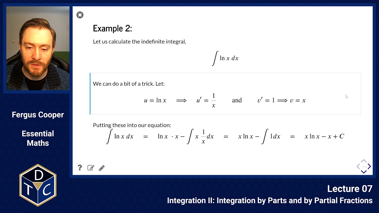
Integration by parts: example 2

Let us calculate the indefinite integral,

\int \ln x\,dx

We can do a bit of a trick. Let:

u=\ln x \quad\Longrightarrow\quad u'=\frac{1}{x}\qquad\text{and}\qquad v'=1\quad\Longrightarrow\quad v=x

Putting these into our equation:

\begin{aligned} \int \ln x\,dx &= \ln x \cdot x - \int x\,\frac{1}{x}\,dx \\ &= x \ln x - \int 1\, dx = x \ln x - x + C \end{aligned}

We can also check this calculation using SymPy:

import sympy as sp
x = sp.symbols('x')
sp.integrate(sp.log(x),x)

x \log{\left(x \right)} - x

(SymPy writes

\log

for the natural logarithm,

\ln

Integration by parts: example 3

\int\limits^{\infty}_0 x^3\,e^{-x}\,dx

Using the formula:

\Big(\int u\, v'\, dx = [u\, v]-\int v\, u'\, dx\Big)

Choose

u=x^3\qquad\text{and}\qquad v'=e^{-x} \qquad\text{so that}\qquad u'=3x^2\qquad\text{and}\qquad v=-e^{-x}

Then:

\int\limits^{\infty}_0 x^3\,e^{-x}\,dx=-\Big[x^3\,e^{-x}\Big]^{\infty}_0 +\int\limits^{\infty}_0 3x^2\,e^{-x}\,dx

Now apply integration by parts to the right-hand side:

Choose

u=3x^2\qquad\text{and}\qquad v'=e^{-x} \qquad\text{so that}\qquad u'=6x\qquad\text{and}\qquad v=-e^{-x}

Then:

\int\limits^{\infty}_0 3x^2\,e^{-x}\,dx=-\Big[3x^2\,e^{-x}\Big]^{\infty}_0 +\int\limits^{\infty}_0 6x\,e^{-x}\,dx

And, once more:

Choose

u=6x\qquad\text{and}\qquad v'=e^{-x} \qquad\text{so that}\qquad u'=6\qquad\text{and}\qquad v=-e^{-x}

Then:

\begin{aligned} \int\limits^{\infty}_0 6x\,e^{-x}\,dx &=-\Big[6x\,e^{-x}\Big]^{\infty}_0 +\int\limits^{\infty}_0 6\,e^{-x}\,dx \\ \Longrightarrow \int\limits^{\infty}_0 6\,e^{-x}\,dx &= -\Big[6\,e^{-x}\Big]^{\infty}_0=0+6e^0=6 \end{aligned}

(Since

e^{-x}\to 0

x\to\infty

, and

e^0=1

)

The other terms are all zero, because

x^3e^{-x}

3x^2e^{-x}

and

6x\,e^{-x}

all tend to

0

x\to\infty

(

e^{-x}

shrinks faster than any power of

x

grows), and all are

0

x=0

\begin{aligned} -\Big[x^3\,e^{-x}\Big]^{\infty}_0 &= 0 - 0 = 0 \\ -\Big[3x^2\,e^{-x}\Big]^{\infty}_0 &= 0 - 0 = 0 \\ -\Big[6x\,e^{-x}\Big]^{\infty}_0 &= 0 - 0 = 0 \end{aligned}

So, to answer our original question:

\int\limits^{\infty}_0 x^3\,e^{-x}\,dx=6

Let's also check it with SymPy:

sp.integrate(x**3 * sp.exp(-x),(x,0,sp.oo))

6

This result actually generalises:

\int\limits^{\infty}_0 x^n\,e^{-x}\,dx=n! \qquad \text{for } n = 0, 1, 2, \ldots

Here

n!

(read "

n

factorial") is the product of the whole numbers from

n

down to 1:

n! = n \times (n-1) \times \cdots \times 2 \times 1

For example,

3! = 3 \times 2 \times 1 = 6

, which is the answer we found above, and by convention

0! = 1

Integration by parts: example 4, trigonometry

Recall that:

\begin{aligned} \frac{d}{dx}(\sin x) &=\cos x \\ \frac{d}{dx}(\cos x) &=-\sin x \end{aligned}

Let's try and calculate the following integral:

\int\limits^b_a \cos x\,e^{-x}\,dx = I

Choose

\begin{aligned} &u=\cos x\qquad\text{and}\qquad v'=e^{-x} \\ \text{so that}\qquad &u'=-\sin x\qquad\text{and}\qquad v=-e^{-x} \end{aligned}

Then:

I =\Big[-\cos x\, e^{-x}\Big]^b_a -\int\limits^b_a (-)\sin x\,(-)e^{-x}\,dx

Next, choose

\begin{aligned} &u=\sin x\qquad\text{and}\qquad v'=e^{-x} \\ \text{so that}\qquad &u'=\cos x\qquad\text{and}\qquad v=-e^{-x} \end{aligned}

Then:

I =\Big[-\cos x\, e^{-x}\Big]^b_a - \Big[\sin x\,(-)e^{-x}\Big]^b_a + \int\limits^b_a \cos x\,(-)e^{-x}\,dx

The last term is the integral we started with:

\Longrightarrow \quad 2\int\limits^b_a \cos x\,e^{-x}\,dx = \Big[\sin x\, e^{-x}\Big]^b_a - \Big[\cos x\, e^{-x}\Big]^b_a

Integration method 3: partial fractions

If we want to calculate the integral below, none of the previous rules allow us to make much progress.

\int \frac{dx}{(2x+1)(x-5)}

But, in this case, we can try splitting the denominator up into two fractions that we can deal with:

\text{Let}\qquad \frac{1}{(2x+1)(x-5)}=\frac{A}{(2x+1)} + \frac{B}{(x-5)}

If we multiply both sides by

(2x+1)(x-5)

, we get:

A(x-5)+B(2x+1)=1 \qquad\text{so}\qquad Ax-5A+2Bx+B=1

We can then equate coefficients of

x

A+2B=0 \qquad\text{thus}\qquad A=-2B \qquad \text{(A)}

Equate the constant terms (coefficients of

x^0

-5A+B=1 \qquad\text{so from (A):}\qquad 10B+B=1, \quad B=\frac{1}{11}, \quad A=-\frac{2}{11}

Thus:

\int \frac{dx}{(2x+1)(x-5)}=-\int \frac{2\, dx}{11(2x+1)} + \int \frac{dx}{11(x-5)}

Now use method of substitution on the first fraction:

u=2x+1

du/dx=2

and

dx/du=1/2

And on the second fraction:

w=x-5

dw/dx=1

and

dx/dw=1

\begin{aligned} -\int \frac{2\, du}{2 \times 11 \times u} + \int \frac{dw}{11w} &= -\frac{\ln |u|}{11} + \frac{\ln |w|}{11} \\ &=-\frac{\ln |2x+1|}{11} + \frac{\ln |x-5|}{11} + C \end{aligned}

SymPy can also solve integrals requiring partial fractions:

sp.integrate(1/((2*x + 1)*(x - 5)),x)

\frac{\log{\left(x - 5 \right)}}{11} - \frac{\log{\left(x + \frac{1}{2} \right)}}{11}

This answer seems different because of the arbitrary constant of integration.

Introductory problems

For more practice, an AI tool can write new problems like the ones below. Ask it for problems of the same type and difficulty, or for problems set in your own field. For example, you could ask it to "write five cell biology problems on integration by parts, at the level of these ones". Work them on paper first, then ask the tool to check your answers and to explain any step you are unsure of.

Introductory problems 1

By using suitable substitutions, evaluate the following integrals:

$\int x^2(x^3+4)^2\,dx$
$\int e^{-x}(5-4e^{-x})\,dx$
$\int (1+x)\sqrt{(4x^2+8x+3)}\,dx$
$\int 3x e^{(x^2+1)}\,dx$

In each case we choose

u

so that

\frac{du}{dx}

appears (up to a constant) in the integrand.

Let $u = x^3+4$ , so $\frac{du}{dx} = 3x^2$ and $x^2\,dx = \frac{1}{3}du$ :
$\int x^2(x^3+4)^2\,dx = \frac{1}{3}\int u^2\,du = \frac{1}{9}u^3 + C = \frac{1}{9}(x^3+4)^3 + C$
Let $u = 5-4e^{-x}$ , so $\frac{du}{dx} = 4e^{-x}$ and $e^{-x}\,dx = \frac{1}{4}du$ :
$\int e^{-x}(5-4e^{-x})\,dx = \frac{1}{4}\int u\,du = \frac{1}{8}u^2 + C = \frac{1}{8}(5-4e^{-x})^2 + C$
Let $u = 4x^2+8x+3$ , so $\frac{du}{dx} = 8x+8 = 8(1+x)$ and $(1+x)\,dx = \frac{1}{8}du$ :
$\begin{aligned} \int (1+x)\sqrt{4x^2+8x+3}\,dx &= \frac{1}{8}\int u^{1/2}\,du = \frac{1}{12}u^{3/2} + C \\ &= \frac{1}{12}(4x^2+8x+3)^{3/2} + C \end{aligned}$
Let $u = x^2+1$ , so $\frac{du}{dx} = 2x$ and $x\,dx = \frac{1}{2}du$ :
$\int 3x e^{(x^2+1)}\,dx = \frac{3}{2}\int e^u\,du = \frac{3}{2}e^{(x^2+1)} + C$

Introductory problems 2

Find the indefinite integrals, with respect to

x

, of the following functions:

$x\,e^{3bx}$
$x^3\,e^{-3x}$
$x \cos (x)$
$e^{bx} \sin(x)$

All four need integration by parts,

\int u\, v'\, dx = [u\, v]-\int v\, u'\, dx

Choose
$\begin{aligned} &u=x\qquad\text{and}\qquad v'=e^{3bx} \\ \text{so that}\qquad &u'=1\qquad\text{and}\qquad v=\frac{1}{3b}e^{3bx} \end{aligned}$
(assuming $b \neq 0$ ). Then:
$\begin{aligned} \int x\,e^{3bx}\,dx &= \frac{x}{3b}e^{3bx} - \int \frac{1}{3b}e^{3bx}\,dx \\ &= \frac{x}{3b}e^{3bx} - \frac{1}{9b^2}e^{3bx} + C \\ &= \frac{e^{3bx}}{3b}\left(x - \frac{1}{3b}\right) + C \end{aligned}$
Here we need to integrate by parts three times, lowering the power of $x$ by one each time. Each time we choose $v'=e^{-3x}$ , so that $v=-\frac{1}{3}e^{-3x}$ :
$\begin{aligned} \int x^3 e^{-3x}\,dx &= -\frac{x^3}{3}e^{-3x} + \int x^2 e^{-3x}\,dx \\ &= -\frac{x^3}{3}e^{-3x} - \frac{x^2}{3}e^{-3x} + \int \frac{2}{3}x e^{-3x}\,dx \\ &= -\frac{x^3}{3}e^{-3x} - \frac{x^2}{3}e^{-3x} - \frac{2x}{9}e^{-3x} + \int \frac{2}{9}e^{-3x}\,dx \\ &= -\frac{x^3}{3}e^{-3x} - \frac{x^2}{3}e^{-3x} - \frac{2x}{9}e^{-3x} - \frac{2}{27}e^{-3x} + C \\ &= -\frac{e^{-3x}}{3}\left(x^3 + x^2 + \frac{2}{3}x + \frac{2}{9}\right) + C \end{aligned}$
Choose
$\begin{aligned} &u=x\qquad\text{and}\qquad v'=\cos(x) \\ \text{so that}\qquad &u'=1\qquad\text{and}\qquad v=\sin(x) \end{aligned}$
Then:
$\int x\cos(x)\,dx = x\sin(x) - \int \sin(x)\,dx = x\sin(x) + \cos(x) + C$
As in the lecture's trigonometry example, we integrate by parts twice and get back the integral we started with. Call it $I$ . First choose
$\begin{aligned} &u=\sin(x)\qquad\text{and}\qquad v'=e^{bx} \\ \text{so that}\qquad &u'=\cos(x)\qquad\text{and}\qquad v=\frac{1}{b}e^{bx} \end{aligned}$
Then:
$I = \frac{1}{b}e^{bx}\sin(x) - \frac{1}{b}\int e^{bx}\cos(x)\,dx$
Next choose $u=\cos(x)$ and $v'=e^{bx}$ , so that $u'=-\sin(x)$ and $v=\frac{1}{b}e^{bx}$ :
$\begin{aligned} I &= \frac{1}{b}e^{bx}\sin(x) - \frac{1}{b}\left(\frac{1}{b}e^{bx}\cos(x) + \frac{1}{b}\int e^{bx}\sin(x)\,dx\right) \\ &= \frac{e^{bx}}{b^2}\big(b\sin(x) - \cos(x)\big) - \frac{1}{b^2}I \end{aligned}$
So, collecting the $I$ terms on the left:
$\begin{aligned} &\left(1 + \frac{1}{b^2}\right)I = \frac{e^{bx}}{b^2}\big(b\sin(x) - \cos(x)\big) \\ \quad\Longrightarrow\quad &I = \frac{e^{bx}\big(b\sin(x) - \cos(x)\big)}{b^2+1} + C \end{aligned}$

Introductory problems 3

Sketch the curve

y=(x-2)(x-5)

and calculate by integration the area between the curve and the

x

-axis, bounded by

x=2

and

x=5

The curve is a parabola, opening upwards, which crosses the

x

axis at

x=2

and

x=5

and the

y

axis at

y=10

. Its minimum is halfway between the roots, at

x=3.5

, where

y=-2.25

. So, between

x=2

and

x=5

the curve lies below the

x

axis.

import numpy as np
from matplotlib import pyplot as plt

x = np.linspace(0, 7, 100)
y = (x - 2) * (x - 5)

plt.plot(x, y)
plt.axhline(0, color='black', linewidth=0.5)
plt.xlabel('x')
plt.ylabel('y')

Expanding,

y = x^2 - 7x + 10

, so:

\int_2^5 (x^2 - 7x + 10)\,dx = \left[\frac{x^3}{3} - \frac{7x^2}{2} + 10x\right]_2^5 = \frac{25}{6} - \frac{26}{3} = -\frac{9}{2}

The integral is negative because the curve is below the axis. The area is its size,

9/2 = 4.5

Introductory problems 4

Use partial fractions to find:

$\int \frac{1}{(x+1)(x+3)}\,dx$
$\int \frac{5x+1}{(x-1)(x+2)}\,dx$
$\int_0^1 \frac{1}{(x+1)(x+2)}\,dx$

Let
$\frac{1}{(x+1)(x+3)} = \frac{A}{x+1} + \frac{B}{x+3}$
Multiplying both sides by $(x+1)(x+3)$ gives $A(x+3) + B(x+1) = 1$ . Equating coefficients of $x$ gives $A + B = 0$ , and equating constant terms gives $3A + B = 1$ . So, $A = 1/2$ and $B = -1/2$ , and
$\begin{aligned} \int \frac{1}{(x+1)(x+3)}\,dx &= \frac{1}{2}\int\frac{dx}{x+1} - \frac{1}{2}\int\frac{dx}{x+3} \\ &= \frac{1}{2}\ln|x+1| - \frac{1}{2}\ln|x+3| + C \end{aligned}$
Let
$\frac{5x+1}{(x-1)(x+2)} = \frac{A}{x-1} + \frac{B}{x+2}$
so that $A(x+2) + B(x-1) = 5x + 1$ . This must hold for every $x$ , so we can also pick values of $x$ that make one term vanish. At $x = 1$ : $3A = 6$ , so $A = 2$ . At $x = -2$ : $-3B = -9$ , so $B = 3$ . So,
$\begin{aligned} \int \frac{5x+1}{(x-1)(x+2)}\,dx &= \int\frac{2}{x-1}\,dx + \int\frac{3}{x+2}\,dx \\ &= 2\ln|x-1| + 3\ln|x+2| + C \end{aligned}$
In the same way, $\frac{1}{(x+1)(x+2)} = \frac{1}{x+1} - \frac{1}{x+2}$ , so
$\begin{aligned} \int_0^1 \frac{1}{(x+1)(x+2)}\,dx &= \Big[\ln|x+1| - \ln|x+2|\Big]_0^1 \\ &= (\ln 2 - \ln 3) - (\ln 1 - \ln 2) \\ &= 2\ln 2 - \ln 3 = \ln\frac{4}{3} \approx 0.288 \end{aligned}$

Main problems

Main problems 1

Evaluate the following indefinite and definite integrals:

$\int 6/(7-x)^3\,dx$
$\int 13x^3(9-x^4)^5\,dx$
$\int_2^5 5\ln(x)\,dx$
$\int x^x\,(1 + \ln(x))\,dx$

Hint for 4.: differentiate

x^x = e^{x\ln(x)}

Let $u = 7-x$ , so $\frac{du}{dx} = -1$ and $dx = -du$ :
$\int \frac{6}{(7-x)^3}\,dx = -\int 6u^{-3}\,du = 3u^{-2} + C = \frac{3}{(7-x)^2} + C$
Let $u = 9-x^4$ , so $\frac{du}{dx} = -4x^3$ and $x^3\,dx = -\frac{1}{4}du$ :
$\begin{aligned} \int 13x^3(9-x^4)^5\,dx &= -\frac{13}{4}\int u^5\,du = -\frac{13}{24}u^6 + C \\ &= -\frac{13}{24}(9-x^4)^6 + C \end{aligned}$
Integrate by parts, as in the lecture's example for $\ln(x)$ . Choose
$\begin{aligned} &u=5\ln(x)\qquad\text{and}\qquad v'=1 \\ \text{so that}\qquad &u'=\frac{5}{x}\qquad\text{and}\qquad v=x \end{aligned}$
Then:
$\begin{aligned} \int_2^5 5\ln(x)\,dx &= \Big[5x\ln(x)\Big]_2^5 - \int_2^5 5\,dx = \Big[5x\ln(x) - 5x\Big]_2^5 \\ &= (25\ln(5) - 25) - (10\ln(2) - 10) \\ &= 25\ln(5) - 10\ln(2) - 15 \approx 18.3 \end{aligned}$
Using the hint and the chain rule:
$\frac{d}{dx}\left(x^x\right) = \frac{d}{dx}\left(e^{x\ln(x)}\right) = e^{x\ln(x)}\,\frac{d}{dx}\big(x\ln(x)\big) = x^x\,(\ln(x) + 1)$
This is exactly the function we are integrating, so
$\int x^x\,(1 + \ln(x))\,dx = x^x + C$

Main problems 2

Suppose the area

A(t)

(in cm

^2

) of a healing wound changes at a rate

\frac{dA}{dt} = -4t^{-3},

where

t

, measured in days, lies between 1 and 10, and the area is

2\,

^2

after 1 day. What will the area of the wound be after 10 days?

Main problems 3

A rocket burns fuel, so its mass decreases over time.

If it burns fuel at a constant rate

\rho\,\text{kg/s}

, and if the exhaust velocity relative to the rocket is a constant

v_e\,\text{m/s}

, then there will be a constant force of magnitude

\rho v_e

propelling it.

The rocket starts burning fuel at

t=0\,\text{s}

with total mass of

m_0\,\text{kg}

, and runs out of fuel at a later time

t=t_f\,\text{s}

, with a final mass of

m_f\,\text{kg}

Newton's second law tells us that the instantaneous acceleration $a$ of the rocket at time $t$ is equal to the force propelling it at that time, divided by its mass at that time. Write down an expression for $a$ as a function of $t$ .
By integrating this expression, show that the rocket's total change in velocity is given by
$v_e \ln\left(\frac{m_0}{m_f}\right).$

The rocket loses mass at the constant rate $\rho$ , starting from $m_0$ , so its mass at time $t$ is $m(t) = m_0 - \rho t$ . So, its acceleration is
$a(t) = \frac{\rho v_e}{m_0 - \rho t}$
Acceleration is the rate of change of velocity, so the total change in velocity is the integral of $a$ from $t=0$ to $t=t_f$ :
$\Delta v = \int_0^{t_f} \frac{\rho v_e}{m_0 - \rho t}\,dt$
Let $u = m_0 - \rho t$ , so $\frac{du}{dt} = -\rho$ and $dt = -\frac{1}{\rho}du$ . When $t=0$ , $u=m_0$ , and when $t=t_f$ , $u=m_f$ :
$\begin{aligned} \Delta v &= -v_e\int_{m_0}^{m_f} \frac{1}{u}\,du = -v_e\Big[\ln(u)\Big]_{m_0}^{m_f} \\ &= -v_e\big(\ln(m_f) - \ln(m_0)\big) = v_e \ln\left(\frac{m_0}{m_f}\right) \end{aligned}$

Main problems 4

The flow of water pumped upwards through the xylem of a tree,

F

, is given by:

F = M_0(p+qt)^{3/4},

where

t

is the tree's age in days,

p

and

q

are positive constants, and

M_0p^{3/4}

is the flow when the tree is planted (i.e. at

t=0

Determine the total volume of water pumped up the tree in its tenth year (ignoring leap years) if:

$p=10$ ,
$q=0.01\,$ day $^{-1}$ , and
$M_0=0.92\,$ l $\,$ day $^{-1}$ .

The volume is the integral of the flow over the tenth year, which runs from day

9 \times 365 = 3285

to day

10 \times 365 = 3650

V = \int_{3285}^{3650} M_0(p+qt)^{3/4}\,dt

Let

u = p + qt

, so

dt = \frac{1}{q}du

V = \frac{M_0}{q}\int u^{3/4}\,du = \left[\frac{4M_0}{7q}(p+qt)^{7/4}\right]_{3285}^{3650}

With the values given,

p+qt

runs from

42.85

46.5

\begin{aligned} V &= \frac{4 \times 0.92}{7 \times 0.01}\left(46.5^{7/4} - 42.85^{7/4}\right) \\ &\approx 52.57 \times (828.02 - 717.65) \approx 5800 \text{ litres} \end{aligned}

Extension problems

Extension problems 1

Express

\frac{1}{x(x^2-16)}\quad\text{in the form}\quad\frac{A}{x} + \frac{B}{(x+4)} + \frac{C}{(x-4)}.

Hence calculate

\int\frac{1}{x(x^2-16)}\,dx.

Since

x^2-16 = (x+4)(x-4)

, we want

\frac{1}{x(x+4)(x-4)} = \frac{A}{x} + \frac{B}{x+4} + \frac{C}{x-4}

Multiply both sides by

x(x+4)(x-4)

1 = A(x+4)(x-4) + Bx(x-4) + Cx(x+4)

This must hold for every

x

, so we can choose convenient values:

$x=0$ gives $1 = -16A$ , so $A = -\frac{1}{16}$
$x=-4$ gives $1 = 32B$ , so $B = \frac{1}{32}$
$x=4$ gives $1 = 32C$ , so $C = \frac{1}{32}$

Therefore:

\frac{1}{x(x^2-16)} = -\frac{1}{16x} + \frac{1}{32(x+4)} + \frac{1}{32(x-4)}

Each term integrates to a logarithm:

\int\frac{1}{x(x^2-16)}\,dx = -\frac{1}{16}\ln|x| + \frac{1}{32}\ln|x+4| + \frac{1}{32}\ln|x-4| + C

The last two terms can also be combined, as

\frac{1}{32}\ln|x^2-16|

Extension problems 2

The speeds of the molecules of mass

m

in a gas at temperature

T

follow the Maxwell-Boltzmann distribution, whose probability density is:

f(v) = 4 \pi \left(\frac{m}{2\pi k T} \right)^{3/2} v^2 e^{-mv^2/2kT}

where

k

is Boltzmann's constant. Find the average speed:

\overline {v} =\int_0^{\infty}v\,f(v)\,dv.

To keep the algebra tidy, write

A = 4 \pi \left(\frac{m}{2\pi k T} \right)^{3/2}

and

B = \frac{m}{2kT}

, so that

\overline{v} = A\int_0^{\infty} v^3 e^{-Bv^2}\,dv

First substitute

w = v^2

, so

\frac{dw}{dv} = 2v

and

v^3\,dv = \frac{1}{2}w\,dw

. The limits stay as

0

and

\infty

\int_0^{\infty} v^3 e^{-Bv^2}\,dv = \frac{1}{2}\int_0^{\infty} w\,e^{-Bw}\,dw

Now integrate by parts, choosing

\begin{aligned} &u=w\qquad\text{and}\qquad v'=e^{-Bw} \\ \text{so that}\qquad &u'=1\qquad\text{and}\qquad v=-\frac{1}{B}e^{-Bw} \end{aligned}

(here

v

is the part in the formula, not the speed). Then:

\begin{aligned} \int_0^{\infty} w\,e^{-Bw}\,dw &= \left[-\frac{w}{B}e^{-Bw}\right]_0^{\infty} + \frac{1}{B}\int_0^{\infty} e^{-Bw}\,dw \\ &= 0 + \frac{1}{B}\left[-\frac{1}{B}e^{-Bw}\right]_0^{\infty} = \frac{1}{B^2} \end{aligned}

(The first term is zero at both ends, since

e^{-Bw}

shrinks faster than

w

grows.) So

\int_0^{\infty} v^3 e^{-Bv^2}\,dv = \frac{1}{2B^2}

, and:

\overline{v} = \frac{A}{2B^2} = 4 \pi \left(\frac{m}{2\pi k T} \right)^{3/2}\frac{2k^2T^2}{m^2} = \frac{4}{\sqrt{2\pi}}\sqrt{\frac{kT}{m}} = \sqrt{\frac{8kT}{\pi m}}

As we might expect, heavier molecules move more slowly on average, and all molecules move faster at higher temperature.

Extension problems 3

Baranov developed expressions for commercial yields of fish in terms of lengths,

L

, of the fish. His formula gave the total number of fish of length

L

k\,e^{-cL}

, where

c

and

k

are constants (

k

and

c

are positive).

Give a sketch of the graph $f(L)=k\,e^{-cL}$ . (Something decreasing, concave upward and asymptotic to horizontal axis will do.) On your sketch, introduce marks on the horizontal axis that represent lengths $L=1$ , $L=2$ , $L=3$ , $L=4$ and $L=5$ . Now draw a rectangle on your sketch that represents the number of fish whose lengths are between $L=3$ and $L=4$ .
Explain how we can represent the total number of fish $N$ as an area. Show that this number equals $k/c$ .
Only fish longer than $L_0$ count as commercial. Hence, assuming that the fish are all similar in shape (i.e. their width and breadth scales with their length) and of equal density $\rho$ , show that the weight, $W$ , of the commercial fish population is
$W= \int_{L_0}^{+\infty} a\, k \rho\,L^3 e^{-cL}\,dL,$
and hence that
$W=\frac{N\, a\, \rho\, e^{-cL_0}}{c^3} \left((cL_0)^3 +3(cL_0)^2+ 6cL_0 +6\right),$
where $a$ is a constant.

The graph starts at $f(0)=k$ on the vertical axis and decreases towards zero as $L$ increases, without ever reaching it. The number of fish with lengths between $L=3$ and $L=4$ is the area under the curve between those two marks, which is close to the area of a rectangle of width 1 and height $f(3.5)$ .
```
import numpy as np
from matplotlib import pyplot as plt

k, c = 1, 0.5
L = np.linspace(0, 8, 100)

plt.plot(L, k * np.exp(-c * L))
plt.bar(3.5, k * np.exp(-c * 3.5), width=1, alpha=0.3)
plt.xlabel('L')
plt.ylabel('f(L)')
```
In the same way, the number of fish with lengths between $L$ and $L + \Delta L$ is about $f(L)\,\Delta L$ . Adding up these strips over all lengths, and letting $\Delta L \to 0$ , gives the total number of fish as the whole area under the curve:
$N = \int_0^{\infty} k\,e^{-cL}\,dL = \left[-\frac{k}{c}e^{-cL}\right]_0^{\infty} = 0 + \frac{k}{c} = \frac{k}{c}$
If the fish are all the same shape, the volume of a fish of length $L$ is proportional to $L^3$ , say $aL^3$ , and its weight is $a\rho L^3$ . The fish with lengths between $L$ and $L + \Delta L$ number about $k\,e^{-cL}\,\Delta L$ , so they weigh about $a\rho L^3\,k\,e^{-cL}\,\Delta L$ . Adding these up over the commercial lengths, $L \geq L_0$ , gives
$W= \int_{L_0}^{\infty} a\, k \rho\,L^3 e^{-cL}\,dL$
To evaluate it, we integrate by parts three times. Each time we choose $v' = e^{-cL}$ , so that $v = -\frac{1}{c}e^{-cL}$ , and each $[u\,v]$ term is zero at infinity:
$\begin{aligned} \int_{L_0}^{\infty} L^3 e^{-cL}\,dL &= \frac{L_0^3}{c}e^{-cL_0} + \frac{3}{c}\int_{L_0}^{\infty} L^2 e^{-cL}\,dL \\ \int_{L_0}^{\infty} L^2 e^{-cL}\,dL &= \frac{L_0^2}{c}e^{-cL_0} + \frac{2}{c}\int_{L_0}^{\infty} L e^{-cL}\,dL \\ \int_{L_0}^{\infty} L e^{-cL}\,dL &= \frac{L_0}{c}e^{-cL_0} + \frac{1}{c}\int_{L_0}^{\infty} e^{-cL}\,dL = \frac{L_0}{c}e^{-cL_0} + \frac{1}{c^2}e^{-cL_0} \end{aligned}$
Putting these together:
$\begin{aligned} \int_{L_0}^{\infty} L^3 e^{-cL}\,dL &= e^{-cL_0}\left(\frac{L_0^3}{c} + \frac{3L_0^2}{c^2} + \frac{6L_0}{c^3} + \frac{6}{c^4}\right) \\ &= \frac{e^{-cL_0}}{c^4}\left((cL_0)^3 +3(cL_0)^2+ 6cL_0 +6\right) \end{aligned}$
From part 2., $k = Nc$ , so
$\begin{aligned} W &= a\,Nc\,\rho\,\frac{e^{-cL_0}}{c^4}\left((cL_0)^3 +3(cL_0)^2+ 6cL_0 +6\right) \\ &= \frac{N\, a\, \rho\, e^{-cL_0}}{c^3} \left((cL_0)^3 +3(cL_0)^2+ 6cL_0 +6\right) \end{aligned}$