OxRSE Training

Gradient descent

One of the simplest local optimisation algorithms is gradient descent. It is initialised at some point in parameter space

a_0

, and at each iteration the function

f(x)

is reduced by following the direction of steepest descent

-\nabla f(a)

a_{n+1} = a_n - \gamma \nabla f(a_n)

This is an example of an important class of algorithms called the line search methods. These algorithms choose a search direction

p_k

at each iteration

k

, and search along the 1D line from the initial point

a_k

to a new point

a_{k+1} = a_k + \alpha p_k

with a lower function value. The problem at each iteration becomes a one-dimensional optimisation problem along

p_k

to find the optimal value of

\alpha

. Each line search algorithm is thus defined on how it chooses both the search direction

p_k

and the optimal

\alpha

Plateaus with low gradient

An obvious downside to simple gradient descent can be seen for functions which have regions of zero or small gradients, or plateaus. Here a gradient descent algorithm with a constant

\gamma

will proceed very slowly, if at all. This motivates another important line search algorithm, Newtons method.

The Newtons direction

p^N_k

can be derived by considering the second-order Taylor expansion of the function

f(x)

f(a_k + p) \approx f(a_k) + p^T \nabla f(a_k) + \frac{1}{2} p^T \nabla^2 f(a_k) p = m_k(p).

We find the value of

p

that minimises

m_k(p)

by setting the derivative of

m_k

to zero, leading to

p_k^N = - (\nabla^2 f(a_k))^{-1} \nabla f(a_k)

Unlike the steepest descent, Newtons method has a natural step length

\alpha \approx 1

, which is suitable for a wide variety of problems and can quickly cross areas of low gradient. Naturally, since the algorithm is based on a second-order approximation of the function

f

, it works better if this approximation is reasonably accurate.

Newtons method can be used as long as the inverse of the second derivative of the function

(\nabla^2 f(a_k))^{-1}

, exists (e.g. it will always exist for a positive definite

\nabla^2 f

). However, even when this inverse does exist it is possible that the direction

p^N_k

does not satisfy the descent condition

f(a_k + \alpha p^N_k) < f(a_k)

(or equivilently

\nabla f(a_k)^T p^N < 0

), so many modifications to Newtons methods, falling under a class of methods called Quasi-Newton methods, have been proposed to satisfy this descent condition.

Quasi-Newton methods do not require the (often onerous) calculation of the hession

\nabla^2 f(x)

like Newtons, instead they form an approximation to the hessian

B_k \approx \nabla^2 f(a_k)

that is updated at each step using the information given by the gradient evaluations

\nabla f(a_k)

. Two popular methods of performing this update are the symmetric-rank-one (SR1), and the Broyden, Fletcher, Goldfarb, and Shanno, (BFGS) formula. Once the approximation

B_k

is formed then the search direction is calculated via

p_k = -B_k^{-1} \nabla f(a_k)

For more details of other line search methods, please see Chapter 3 of the Nocedal and Wright textbook, or in the other textbooks listed at the end of this lesson. Finally, it should be noted that the conjugate gradient method can also be used for non-linear optimisation, where the search direction is given by

p_k = -\nabla f(a_k) + \beta_k p_{k-1}

Step length

In line search methods, choosing the step length

\alpha_k

is a non-trivial task. Ideally we would want to chose

\alpha_k

to minimise the function along the one-dimensional search direction

p_k

. That is, we wish to minimise

\phi(\alpha_k) = f(a_k + \alpha_k p_k),\text{ }\alpha_k > 0.

In general it is too expensive to do this minimisation exactly, so approximate methods are used so that multiple trial

\alpha_k

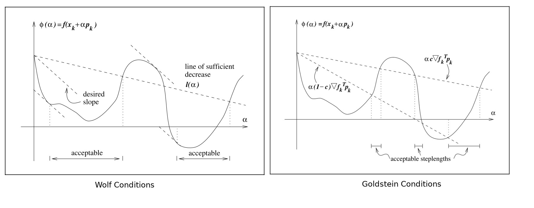
values are trialled, stopping when a candidate is found that satisfies a set of conditions. There are two main conditions used, the Wolfe conditions and the Goldstein conditions.

The two Wolfe conditions are the sufficient decrease condition, which ensures that the reduction in the function value is proportional to the step length

\alpha_k

and the gradient in the direction of the step

f(a_k + \alpha_k p_k) \le f(a_k) + c_1 \alpha_k \nabla f(a_k)^T p_k.

The second Wolfe condition is the curvature condition, which prevents unacceptibly short steps by ensuring that the slope of

\phi

is greater than some constant

c_2

times the initial slope

\phi'(0)

\nabla f(a_k + \alpha_k p_k)^T p_k \ge c_2 \nabla f(a_k)^T p_k,

where

c_2 \in (c_1, 1)

. Typical values are

c_1 = 10^{-4}

and

c_2 = 0.9

. The strong Wolfe conditions restrict the gradient

\phi'

to be small, so as to exclude points that are too far from stationary points of

\phi

f(a_k + \alpha_k p_k) \le f(a_k) + c_1 \alpha_k \nabla f(a_k)^T p_k.

|\nabla f(a_k + \alpha_k p_k)^T p_k| \le c_2 |\nabla f(a_k)^T p_k|,

The Goldstein conditions are similar in spirit to the Wolfe conditions, and are formed from the two inequalities

f(a_k) + (1 - c) \alpha_k \nabla f(a_k)^T p_k \le f(a_k + \alpha_k p_k) \le f(a_k) + c \alpha_k \nabla f(a_k)^T p_k.

with

0 < c < 1/2

. The first inequality prevents small step sizes while the second is the same sufficient decrease condition as in the Wolfe conditions. The Goldstein conditions are often used in Newton-type methods but for quasi-Newton methods the Wolfe conditions are prefered. The diagrams from the text by Nocedal and Wright illustrate the two conditions

Algorithms for choosing candidate step size values

\alpha_k

can be complicated, so we will only mention here one of the simplest, which is the backtracking method. This approach implicitly satisfies the condition on too small

\alpha_k

, and only repeatedly test for the common sufficient decrease condition that appears in both the Wolfe and Goldstein condtitions.

Backtracking algorithm

Choose

\bar{\alpha} > 0

\rho \in (0, 1)

c \in (0, 1)

\alpha_k := \bar{\alpha}

repeat until

f(a_k + \alpha_k p_k) \le f(a_k) + c \alpha_k \nabla f(a_k)^T p_k

$\alpha_k := \rho \alpha_k$

end repeat.

Software

Scipy has a wide variety of (mostly) line search and trust region algorithms in scipy.optimize. There are 14 local minimisers, so we won't list them all here!
It is worth noting that Scipy includes the line_search function, which allows you to use their line search satisfying the strong Wolfe conditions with your own custom search direction.
Scipy also includes a HessianUpdateStrategy, which provides an interface for specifying an approximate Hessian for use in quasi-Newton methods, along with two implementations BFGS and SR1.

Problems

Line Search Problems

Program the steepest descent and Newton algorithms using the backtracking line search. Use them to minimize the Rosenbrock function. Set the initial step length $\alpha_0 = 1$ and print the step length used by each method at each iteration. First try the initial point $x_0 = (1.2, 1.2)^T$ and then the more difficult starting point $x_0 = (−1.2, 1)^T$ .
Plot the function surface using matplotlib and overlay the line search segments so you can visualise the progress of your algorithm. Observe the difference between the algorithms when the gradient of the rosenbrock function is low (i.e. at the bottom of the curved valley)
Repeat (1) and (2) above using the line search implemented in Scipy scipy.optimize.line_search, which uses the strong Wolfe conditions.

import numpy as np
from matplotlib import cm
import scipy.optimize
from matplotlib import pyplot as plt

def steepest_descent(x, f, grad_f, hessian_f):
    return -grad_f(x)

def newton(x, f, grad_f, hessian_f):
    A = hessian_f(x)
    return -np.linalg.solve(A, grad_f(x))

def backtracking(f, grad_f, x, p):
    alpha = 1.0
    c = 1e-4
    rho = 0.5
    f_x = f(x)
    c_grad_f_x_p = c*grad_f(x).dot(p)
    while f(x + alpha*p) > f_x + alpha * c_grad_f_x_p:
        alpha = rho * alpha
    return alpha

def scipy_line_search(f, grad_f, x, p):
    return scipy.optimize.line_search(f, grad_f, x, p)[0]

def minimise(f, grad_f, hessian_f, x0, tol=1e-5, max_iter=1000, search_direction=steepest_descent, line_search=backtracking):
    x = np.copy(x0)
    alpha = 1.0
    p = np.zeros_like(x)
    p[0] = 1.
    i = 0
    array_x = np.empty((max_iter+1, len(x)), dtype=float)
    array_alpha = np.empty(max_iter, dtype=float)
    array_x[0, :] = x
    while np.linalg.norm(alpha * p) > tol and i < max_iter:
        p = search_direction(x, f, grad_f, hessian_f)
        alpha = line_search(f, grad_f, x, p)
        x += alpha * p
        array_x[i+1, :] = x
        array_alpha[i] = alpha
        i += 1
    return array_x[:i,:], array_alpha[:i]

def rosenbrock(x, y):
    return (1 - x)**2 + (y - x**2)**2

def rosenbrock_2d(x):
    return (1 - x[0])**2 + (x[1] - x[0]**2)**2

def grad_rosenbrock_2d(x):
    return np.array([
        4*x[0] * (x[0]**2 - x[1]) + 2*x[0] - 2,
        -2*x[0]**2 + 2*x[1]
    ])

def hessian_rosenbrock_2d(x):
    return np.array([
        [12 * x[0]**2 - 4*x[1] + 2, -4*x[0]],
        [-4*x[0], 2],
    ])

# verify grad and hessian using finite differences
h = 1e-5
x0 = np.array([0., 0.])
x0_x = np.array([h, 0.])
x0_y = np.array([0., h])
fd_grad_rosenbrock = np.array([
    (rosenbrock_2d(x0_x) - rosenbrock_2d(x0)) / h,
    (rosenbrock_2d(x0_y) - rosenbrock_2d(x0)) / h,
])
np.testing.assert_almost_equal(fd_grad_rosenbrock, grad_rosenbrock_2d(x0), decimal=4)
fd_hessian_rosenbrock = np.vstack((
    (grad_rosenbrock_2d(x0_x) - grad_rosenbrock_2d(x0)) / h,
    (grad_rosenbrock_2d(x0_y) - grad_rosenbrock_2d(x0)) / h,
))
np.testing.assert_almost_equal(fd_hessian_rosenbrock, hessian_rosenbrock_2d(x0),
                               decimal=4)

# plot rosenbrock surface
x = np.linspace(-1.5, 2.0, 100)
y = np.linspace(0.2, 3.0, 100)
X, Y = np.meshgrid(x, y)
Z = np.vectorize(rosenbrock)(X, Y)

fig = plt.figure()
ax = fig.gca(projection='3d')
fig2 = plt.figure()
ax2 = fig2.add_subplot(1,1,1)

surf = ax.plot_surface(X, Y, Z, alpha=0.5, cmap=cm.coolwarm)

# pick two initial starting points
x01 = np.array([1.2, 1.2])
x02 = np.array([-1.2, 1])

# run all methods and plot results
for x0 in [x01, x02]:
    for p_method in [steepest_descent, newton]:
        for ls_method in [backtracking, scipy_line_search]:
            label = '{}-{}'.format(p_method.__name__, ls_method.__name__)
            pos, alpha = \
                minimise(rosenbrock_2d, grad_rosenbrock_2d, hessian_rosenbrock_2d, x0,
                         search_direction=p_method, line_search=ls_method)
            print('method', label, 'finished in', len(alpha), 'iterations')
            xs = pos[:, 0]
            ys = pos[:, 1]
            ax.plot(xs, ys, rosenbrock(xs, ys), label=label, linewidth=2)
            ax2.plot(alpha, label=label)
ax2.legend()
plt.show()

Line Search Methods