OxRSE Training

In these exercises we will use Python to solve a variety of Ordinary Differential Equations (ODEs), including initial and boundary value problems. Prior to attempting the exercises you should be familiar with how to solve first order ODEs using separable solutions and integrating factors. You should also know how solve a second order ODE with constant coefficients and how to reduce a general second order ODE to a system of coupled first order equations. If you are not familiar with this material then speak to a module leader or demonstrator who will give you a tutorial. Advanced exercises are marked with a star (

\star

); you should attempt these only if you have time and have completed the other exercises.

Motivation

Ordinary differential equations are used very frequently in modelling biological and physiological processes. Most commonly they are used to model the way in which quantities of interest (such as concentrations of drugs, viral load, or population densities) change as a function of time. The earlier exercises below are revision of the kinds of ODEs you may have encountered at A level or as an undergraduate. The later exercises are taken from real models of chemical and biological systems.

The intentions behind this exercise are:

To give you a clear goal to meet
To give you a chance to revise or learn a few things. Specifically:
- The abstract base class pattern;
- Unit testing with unittest;
- Ordinary differential equation solver implementations.

A nice feature of this assignment is that you are provided with a testing infrastructure which gives an implicit specification of the code you are required to write. This means that when you've written code such that all the tests pass then you will know that you have completed the exercise.

Initial value problems

Solve the following initial value problems by hand:

$\dfrac{\textrm{d} y}{\textrm{d} x} = x^{2}$ , $\;$ subject to $y(0)=1$ .
$\dfrac{\textrm{d} x}{\textrm{d} t} = \dfrac{t^{2}}{x}$ , $\;$ subject to $x(0)=1$ .
$\dfrac{\textrm{d} y}{\textrm{d} x} + \dfrac{y}{x}=1$ , $\;$ subject to $y(1)=0$ .
$\dfrac{\textrm{d} y_{1}}{\textrm{d} x} = -y_{2}$ and $\dfrac{\textrm{d} y_{2}}{\textrm{d} x} = y_{1}$ , $\;$ subject to $y_{1}(0)=1$ and $y_{2}(0)=0$ .
$\dfrac{\textrm{d}^{2} y}{\textrm{d} x^{2}} +3\dfrac{\textrm{d} y}{\textrm{d} x} -4y=0$ , $\;$ subject to $y(0)=1$ and $y'(0)=0$ .

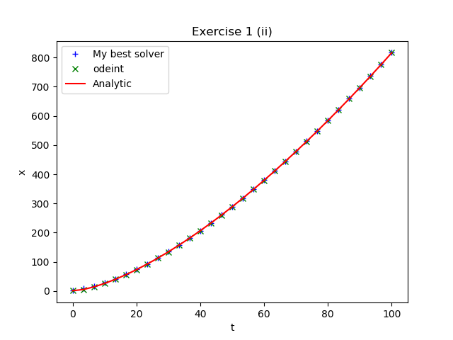
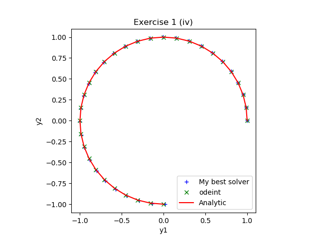
Solve each of the above initial value problems numerically using your best Python ODE solver and compare with the analytic solutions. Note that in order to solve the last problem numerically you will need to reformulate the equation as a system of first order ODEs. See if, for some of your answers, you can make a figure similar to those below, made using model solutions.

The analytical solutions to the initial value problems are given as follows:

$\dfrac{\textrm{d} y}{\textrm{d} x} = x^{2}$ , $y(0)=1$ $\;$ $\Rightarrow$ $\;$ $y(x)=\frac{x^{3}}{3}+1.$ }
$\dfrac{\textrm{d} x}{\textrm{d} t} = \dfrac{t^{2}}{x}$ , $x(0)=1$ $\;$ $\Rightarrow$ \ $x(t)=\sqrt{\frac{2t^{3}}{3}+1}.$
$\dfrac{\textrm{d} y}{\textrm{d} x} + \dfrac{y}{x}=1$ , $y(1)=0$ $\;$ $\Rightarrow$ $\;$ $y(x)=\frac{x}{2}-\frac{1}{2x}.$
$\dfrac{\textrm{d} y_{1}}{\textrm{d} x} = -y_{2}$ , $\dfrac{\textrm{d} y_{2}}{\textrm{d} x} = y_{1}$ , $y_{1}(0)=1$ , $y_{2}(0)=0$ $\;$ $\Rightarrow$ $\;$ $y_{1}(x)=\cos{x}, \; y_{1}(x)=\sin{x}.$
$\dfrac{\textrm{d}^{2} y}{\textrm{d} x^{2}} +3\dfrac{\textrm{d} y}{\textrm{d} x} -4y=0$ , $y(0)=1$ , $y'(0)=0$ $\;$ $\Rightarrow$ $\;$ $y(x)=\frac{4}{5}e^{x}+ \frac{1}{5}e^{-4x} .$

The following example Python codes can be modified to solve all the above initial value problems:

""" Code for question (ii) """
from matplotlib import pyplot as plt
from scipy.integrate import odeint
import numpy as np
import matplotlib.pyplot as plt
# Function to solve dxdt=tˆ2/x.
def dxdtfor2dsolver(u, t):
    # dxdt=t*t/x (dydt is unused)
    return (t*t/u[0], 0)
def dxdt(x, t):
    # dxdt=t*t/x
    return t*t/x

# My best solver
solver = HigherOrderOdeSolver()
solver.SetInitialValues(1, 42)
solver.SetInitialTimeNumberOfStepsAndFinalTime(0.0, 30, 100.0)
solver.SetRhsFunction(dxdtfor2dsolver)
solver.Solve()

# odeint based on the time-steps in my solver
oi = odeint(dxdt, 1.0, solver.GetTimeTrace())

# the analytic version based on the time-steps in my solver
t = solver.GetTimeTrace()
analytic = np.sqrt((np.power(t, 3)*2)/3 + 1.0)

plt.plot(solver.GetTimeTrace(),solver.GetXTrace(),'b+',
         label='My best solver')
plt.plot(solver.GetTimeTrace(), oi, 'gx', label='odeint')
plt.plot(solver.GetTimeTrace(), analytic, 'r', label='Analytic')
plt.legend()
plt.title('Exercise 1 (ii)')
plt.xlabel('t')
plt.ylabel('x')
plt.show()

""" Code for question (iv) """
from matplotlib import pyplot as plt
from scipy.integrate import odeint
import numpy as np
import matplotlib.pyplot as plt
import math
def dydx(y, x):
    # This one ought to look familiar (rhs_circle)
    return (-y[1], y[0])

# My best solver
solver = HigherOrderOdeSolver()
solver.SetInitialValues(1, 0)
solver.SetInitialTimeNumberOfStepsAndFinalTime(0.0, 30, 1.5*math.pi)
solver.SetRhsFunction(dydx)
solver.Solve()

# odeint based on the time-steps in my solver
oi = odeint(dydx, (1,0), solver.GetTimeTrace())

# the analytic version based on the time-steps in my solver
t = solver.GetTimeTrace()
x = solver.GetXTrace()
y = solver.GetYTrace()
analyticx = np.cos(t)
analyticy = np.sin(t)

plt.plot(solver.GetXTrace(), solver.GetYTrace(), 'b+',
         label='My best solver')
plt.plot(oi[:,0], oi[:,1], 'gx', label='odeint')
plt.plot(analyticx,  analyticy, 'r', label='Analytic')
plt.legend()
plt.title('Exercise 1 (iv)')
plt.xlabel('y1')
plt.ylabel('y2')
plt.axes().set_aspect('equal')
plt.show()

Boundary value problems

Use scipy.integrate.solve_bvp to solve the boundary value problem

\begin{aligned} \dfrac{\textrm{d}^{2} y}{\textrm{d} x^{2}} + 3 \dfrac{\textrm{d} y}{\textrm{d} x} -4y=0, \end{aligned}

subject to the boundary conditions

y(0)=1

and

y(1)=1

Solve the same boundary value problem, but now with the boundary conditions

y'(0) = 0

and

y(1)=1

from scipy.integrate import solve_bvp
import matplotlib.pyplot as plt
import numpy as np
# Solving y'' + 3y'- -4y
# y[0] is y, y[1] is y'
# dy[0]/dx = y[1] and dy[1]/dx = -3y[1]+4y[0]
def dydx(x, y):
    return np.vstack((y[1], -3*y[1]+4*y[0]))

def bcs_a(yat0, yat1):
    # Dirichlet: y at both ends = 1, i.e. y(x=1)-1 = 0
    return (yat0[0]-1, yat1[0]-1)
def bcs_b(yat0, yat1):
    # Dirichlet/Neumann y'(x=0)= 1, y(x=1)-1 = 0
    return (yat0[1]-1, yat1[0]-1)

x = np.linspace(0, 1, 50)
init_y = np.ones((2, x.size))
sol_a = solve_bvp(dydx, bcs_a, x, init_y)
sol_b = solve_bvp(dydx, bcs_b, x, init_y)
plt.plot(sol_a.x, sol_a.y[0], 'b-+', label='(a)')
plt.plot(sol_b.x, sol_b.y[0], 'r-*', label='(b)')
plt.title('Exercise (a)')
plt.legend()
plt.xlabel('x')
plt.ylabel('y')
plt.show()

Chemical reaction systems

Mathematical models of simple chemical or biochemical reaction mechanisms often take the form of non-linear systems of ordinary differential equations (derived using the standard chemical laws of mass action). Often the various reactions making up the system happen on very different time scales leading to a stiff system. An example is Robertson's chemical reaction model, in which the concentrations of three reacting chemical species evolve according to the system of equations

\begin{aligned} \dfrac{\textrm{d} y_{1}}{\textrm{d} x} &= -0.04y_1 + 10000 y_2 y_3, \\ \dfrac{\textrm{d} y_{2}}{\textrm{d} x} &=0.04y_1 - 10000 y_2 y_3 - 30000000y_2^2,\\ \dfrac{\textrm{d} y_{3}}{\textrm{d} x} &= 30000000y_2^2, \end{aligned}

with initial conditions

\begin{aligned} y_1(0) = 1, \; y_2(0) = 0, \; y_3 (0) = 0. \end{aligned}

Note: your mileage may vary with this question, because with more modern versions of scipy it becomes increasingly hard to stop the integration scheme being "clever" and using a sophisticated scheme earlier.

Read the documentation for scipy.integrate.ode. Solve this system using the Dormand & Prince dopri solver, which is a high-order Runge-Kutta solver, until $t=100$ in steps of $\Delta t=1$ . (Note that the interface is a bit more difficult to set up than odeint but an example is given with the documentation.) What warning do you get from the solver? Can you change any of the dopri parameters to get rid of warnings? How long does the integrator take to solve the system?
If you are still getting warnings for the dopri then you will have a hint to help you select a better scipy.integrate.ode method. Switch to such a method. Again work to remove all warnings.
( $\star$ ) Explain what is happening mathematically and chemically.
Repeat parts (a)--(b) for the system
$\begin{aligned} \dfrac{\textrm{d} y_{1}}{\textrm{d} x} &= -0.04y_1 + y_2 y_3, \\ \dfrac{\textrm{d} y_{2}}{\textrm{d} x} &=0.04y_1 - y_2 y_3 - 30y_2^2,\\ \dfrac{\textrm{d} y_{3}}{\textrm{d} x} &= 30y_2^2, \end{aligned}$
with the same initial conditions. Which solver is faster now?
Which solver gives you warnings now?
Which solver should you use in which situation?
( $\star$ ) If you are feeling brave then assess how one of the fixed time-step solvers you have written yourself measures up to the solver you used in part (b). There are 3 species so you may want to extend the functionality to cope with $y_3$ . Use the solution from part (b) as a reference to measure your error. How small do you need to make your time-step to get within a particular error?

Code for all parts of this question is given below.

To answer part (c) there is a large discrepancy between numerical values (or concentrations) so effects are occurring on different scales. The proper term for this is multiscale but in ODEs we often call these systems "stiff". Problems arise a little after the initial time when there is a small amount of

y_2

which leads to massive gradients.

Therefore, to answer part (e), for problems occurring on single scales it is okay to use Runge-Kutta type solvers but for problems defined on multiple scales you should use adaptive stiff solvers.

import matplotlib.pyplot as plt
import time
from scipy.integrate import ode

def Robertson(t, Y):
    dYdt = [-0.04*Y[0] + 10000*Y[1]*Y[2],
         0.04*Y[0] - 10000*Y[1]*Y[2] - 30000000*Y[1]**2,
         30000000*Y[1]**2]
    return dYdt

def SimpleODE(t, Y):
    dYdt = [-0.04*Y[0] + Y[1]*Y[2],
         0.04*Y[0] - Y[1]*Y[2] - 30*Y[1]**2,
         30*Y[1]**2]
    return dYdt


t=0
y=[1,0,0]
times=[t]
y1=[1]
y2=[0]
y3=[0]

# Experiments for part (a)
solver = ode(Robertson).set_integrator('dopri')
# UserWarning: dopri5: larger nmax is needed
solver = ode(Robertson).set_integrator('dopri', max_step=1e-6)
# dopri5: larger nmax is needed      0.7 sec WRONG
solver = ode(Robertson).set_integrator('dopri', nsteps=100)
# dopri5: larger nmax is needed       0.2 sec
solver = ode(Robertson).set_integrator('dopri', nsteps=1000)
# dopri5: larger nmax is needed       1.5 sec
solver = ode(Robertson).set_integrator('dopri', nsteps=10000)
# dopri5: problem is probably stiff   1.5 sec


# Experiments for part (b) (FIND A STIFF SOLVER)
solver = ode(Robertson)
# Fails with  "vode: Excess work done on this call." and other messages
solver = ode(Robertson).set_integrator('vode', method='bdf')
# vode: Excess work done on this call
solver = ode(Robertson).set_integrator('vode', method='bdf', nsteps=1000)
# vode: Excess work done on this call
solver = ode(Robertson).set_integrator('vode', method='bdf', nsteps=8000)
# No warnings!            2.2 sec


# Experiments for part (d)
solver = ode(SimpleODE)
# ~6 ms
solver = ode(SimpleODE).set_integrator('dopri')
# ~3 ms
solver = ode(SimpleODE).set_integrator('dopri', nsteps=1000)
# ~3 ms
solver = ode(SimpleODE).set_integrator('vode', method='bdf')
# ~2 ms
solver = ode(SimpleODE).set_integrator('vode', method='bdf', nsteps=8000)
# ~2 ms
# (They all succeed and take a similar amount of time)

solver.set_initial_value(y,t)

start_time = time.time()
while t<100:
    t=t+1
    y=solver.integrate(t)
    y1.append(y[0])
    y2.append(y[1])
    y3.append(y[2])
    times.append(t)
print('Time taken =',time.time()-start_time)
plt.plot(times, y1, label='y1')
plt.plot(times, y2, label='y2')
plt.plot(times, y3, label='y3')
plt.legend()
plt.xlabel('t')
plt.show()

When Zombies Attack!

(

\star

)Inspired by a famous SIR model for epidemics there is a SZR model for zombie invasion. The paper describing this model is available to download from https://mysite.science.uottawa.ca/rsmith43/Zombies.pdf which includes modelling code in Matlab.

A more advanced model included in the paper, which includes latent infection and quarantine, is known as the SIZRQ model. This model is defined by

\begin{aligned} \dfrac{\textrm{d} S}{\textrm{d} t} &= \Pi - \beta SZ - \delta S, \\ \dfrac{\textrm{d} I}{\textrm{d} t} &= \beta S Z -\rho I - \delta I - \kappa I, \\ \dfrac{\textrm{d} Z}{\textrm{d} t} &= \rho I + \zeta R - \alpha S Z -\sigma Z, \\ \dfrac{\textrm{d} R}{\textrm{d} t} &= \delta S + \delta I + \alpha SZ -\zeta R + \gamma Q, \\ \dfrac{\textrm{d} Q}{\textrm{d} t} &= \kappa I +\sigma Z - \gamma Q, \end{aligned}

with initial conditions

\begin{aligned} S(0) = 500, \; I(0) = 0, \; Z(0) = 0, \; R(0) = 0, \; Q(0) = 0 \end{aligned}

and parameter values

\begin{aligned} \Pi = 0, \; \alpha = 0.005, \; & \beta = 0.0095, \; \zeta = 0.1, \; \delta = 0.0001, \\ \rho = 0.5, \; & \kappa = 0.1, \; \sigma = 0.01, \; \gamma = 0.01. \end{aligned}

Solve this system of equations numerically.
How realistic is this type of model? Can you think of any improvements to the model?

import numpy as np
from scipy.integrate import odeint
# Function to solve the SIZRQ Zombie ODE system.
alpha = 0.005
zeta = 0.1
rho = 0.5
sigma = 0.01
pi = 0
beta = 0.0095
delta = 0.0001
kappa = 0.1
gamma = 0.01

def Zombie(Y, t):
    S = Y[0]
    I = Y[1]
    Z = Y[2]
    R = Y[3]
    Q = Y[4]
    dSdt = pi - beta*S*Z - delta*S  # Susceptible
    dIdt = beta*S*Z - rho*I - delta*I - kappa*I # Infected
    dZdt = rho*I + zeta*R - alpha*S*Z - sigma*Z # Zombie
    dRdt = delta*S + delta*I + alpha*S*Z - zeta*R + gamma*Q # Removed
    dQdt = kappa*I + sigma*Z - gamma*Q # Quarantined
    return [dSdt, dIdt, dZdt, dRdt, dQdt]

S0=500
I0=Z0=R0=Q0=0
StartTime=0
EndTime = 50
t = np.linspace(StartTime, EndTime, 100)
Y = odeint(Zombie, [S0,I0,Z0,R0,Q0], t)

plt.plot(t,Y[:,0], label='Susceptible')
plt.plot(t,Y[:,1], label='Infected')
plt.plot(t,Y[:,2], label='Zombie')
plt.plot(t,Y[:,3], label='Removed')
plt.plot(t,Y[:,4], label='Quarantined')

plt.legend()
plt.title('When zombies attack')
plt.xlabel('time')
plt.show()

Possible improvements include the incorporation of delays, spatial heterogeneity, and more realistic nonlinear interaction terms.

Simple events

(

\star

)ODE-based models of biological systems often include specific events, which may occur either at predetermined times or when a given condition on the values of the state variables or their derivatives is met. The following model describes a zombie outbreak in which there is periodic culling (Spoiler alert. It looks like we all die whatever we do. If you think that's depressing then you might have to read this followup paper). of the zombie population:

\begin{aligned} \dfrac{\textrm{d} S}{\textrm{d} t} &= \Pi - \beta SZ - \delta S, & \; t &\ne t_{n} ,\\ \dfrac{\textrm{d} Z}{\textrm{d} t} &= \beta SZ + \zeta R - \alpha S Z, & t &\ne t_{n}, \\ \dfrac{\textrm{d} R}{\textrm{d} t} &= \delta S + \alpha SZ -\zeta R, & t &\ne t_{n}, \\ \triangle Z &= -kZ, & t &= t_{n}. \end{aligned}

Here

k\in(0,1]

is the kill ratio, and the last equation represents periodic culling of the zombie population.

Solve this model subject to initial conditions

\begin{aligned} S(0) = 500, \; Z(0) = 0, \; \text{and} \; R(0) = 0, \end{aligned}

and with parameter values

\begin{aligned} \Pi = 0, \; \alpha = 0.005, \; \beta = 0.0095, \; \zeta = 0.1, \; \delta = 0.0001, \; k = 0.25, \end{aligned}

and culling every 10 units of time (i.e.

t_1=10

t_2=20

, etc.). Hint: you will need to loop over time intervals to solve this model.

import numpy as np
from scipy.integrate import odeint
# Function to solve the SZR Zombie ODE system with culling.
alpha = 0.005
zeta = 0.1
pi = 0
beta = 0.0095
delta = 0.0001

def SZR(Y,t):
    S = Y[0]
    Z = Y[1]
    R = Y[2]
    # Susceptible / Zombie / Removed
    dSdt = pi - beta*S*Z - delta*S
    dZdt = beta*S*Z + zeta*R - alpha*S*Z
    dRdt = delta*S + alpha*S*Z - zeta*R
    return [dSdt, dZdt, dRdt]


S0=500
Z0=0
R0=0
EndTime = 50
CullEffect = 0.30
CullInterval = 10.0
NumCull = round(EndTime/CullInterval)

Y0 = [S0, Z0, R0]
for i in range(0, NumCull):
    t = np.linspace(CullInterval*i, CullInterval*(i+1), 100)
    Y = odeint(SZR, Y0, t)
    # Get state at end
    Y0 = Y[-1,:]
    CullSize = CullEffect*Y0[1]
    Y0[1] -= CullSize
    Y0[2] += CullSize
    plt.plot(t,Y[:,0], 'r', label='Susceptible')
    plt.plot(t,Y[:,1], 'g', label='Zombie')
    plt.plot(t,Y[:,2], 'b', label='Removed')
plt.legend()
plt.title('Zombie culling at '+str(CullEffect*100)+'%')
plt.xlabel('time')
plt.show()
# Turn that graph on its side and you have a Christmas tree!

ODE Solvers - PM Exercises