This material has been adapted from material by Fergus Cooper and others from the "Essential Mathematics" module at the Doctoral Training Centre, University of Oxford.
This course material was developed as part of UNIVERSE-HPC, which is funded through the SPF ExCALIBUR programme under grant number EP/W035731/1
Differentiation 3
Learning outcomes
Be able to calculate the derivative of exponential and logarithmic functions
Understand how to differentiate functions of multiple independent variables
Be able to calculate higher order derivatives with respect to multiple variables
YouTube lecture recording from October 2020
The following YouTube video was recorded for the 2020 iteration of the course.
The material is still very similar:
Exponentials and Partial Differentiation
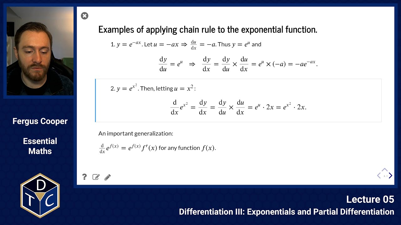
Examples of applying chain rule to the exponential function
y=e−ax
Let u=−ax⇒dxdu=−a.
Thus y=eu and
dudy=eu⇒dxdy=dudy×dxdu=eu×(−1.=−ae−ax.
y=ex2
Then, letting u=x2
dxdex2=dxdy=dudy×dxdu=eu⋅2x=ex2⋅2x.
So an important generalization is:
dxdef(x)=ef(x)f′(x) for any function f(x)
Example with the natural logarithm
y=ln(a−x)2=2ln(a−x)=2lnu.
Let u=(a−x):
⇒dxdu=−1anddudy=u2Thusdxdy=u2×(−1)=a−x−2
This also generalises:
dxdln(f(x))=f(x)f′(x)
The Derivative of ax
By the properties of logarithms and indices we have
ax=(elna)x=e(x⋅lna).
Thus, as we saw above we have:
dxdax=dxde(x⋅lna)=e(x⋅lna)dxd(x⋅lna)=ax⋅lna
Similarly, in general:
dxdaf(x)=af(x)⋅lna⋅f′(x)
Sympy Example
Let's try and use Sympy to demonstrate this:
import sympy as sp
x, a = sp.symbols('x a')# declare the variables x and af = sp.Function('f')# declare a function dependent on another variablesp.diff(a**f(x),x)# write the expression we wish to evaluate
af(x)log(a)dxdf(x)
The Derivative of logax
Recall the conversion formula logax=lnalnx
and note that lna is a constant.
Thus:
x, a = sp.symbols('x a')# declare the variables x and af = sp.Function('f')# declare a function dependent on another variablesp.diff(sp.log(f(x),a),x)# write the expression we wish to evaluate
f(x)log(a)dxdf(x)
Further examples
Product Rule: Let y=x2ex. Then:
dxdy=dxdx2ex=dxdx2⋅ex+x2⋅dxdex=(2x+x2)ex
Quotient Rule: Let y=xex. Then:
dxdy=x2dxdex⋅x−ex⋅dxdx=x2ex⋅x−ex⋅1=x2x−1ex
Chain Rule: y=ex2. Then, letting f(x)=x2:
dxdex2=ef(x)f′(x)=ex2⋅2x
y=ln(x2+1). Then, letting f(x)=x2+1:
dxdln(x2+1)=f(x)f′(x)=x2+12x
dxd2x3=2x3⋅ln2⋅3x2
dxd10x2+1=10x2+1⋅ln10⋅2x
dxdlog10(7x+5)=(7x+5)⋅ln107
dxdlog2(3x+x4)=ln2⋅(3x+x4)3x⋅ln3+4x3
Functions of several variables: Partial Differentiation
Definition: Given a function z=f(x,y) of two variables x and y, the partial derivative of z with respect to x is the function obtained by differentiating f(x,y) with respect to x, holding y constant.
We denote this using ∂ (the "curly" delta, sometimes pronounced "del") as shown below:
∂x∂z=∂x∂f(x,y)=fx(x,y)
Example 1
f(x,y)=z=x2−2y2 > fx=∂x∂z=2xandfy=∂y∂z=−4y
Example 2
Let z=3x2y+5xy2. Then the partial derivative of z with respect to x, holding y fixed, is:
∂x∂z=∂x∂(3x2y+5xy2) > =3y⋅2x+5y2⋅1 > =6xy+5y2
while the partial of z with respect to y holding x fixed is:
∂y∂z=∂y∂(3x2y+5xy2) > =3x2⋅1+5x⋅2y=3x2+10xy
Sympy example
In the previous slide we had:
∂x∂(3x2y+5xy2)=6xy+5y2
Let's redo this in Sympy:
x, y = sp.symbols('x y')sp.diff(3*x**2*y +5*x*y**2,x)
6xy+5y2
Higher-Order Partial Derivatives
Given z=f(x,y) there are now four distinct possibilities for the
second-order partial derivatives.
With respect to x twice:
∂x∂(∂x∂z)=∂x2∂2z=zxx
With respect to y twice:
∂y∂(∂y∂z)=∂y2∂2z=zyy
First with respect to x, then with respect to y:
∂y∂(∂x∂z)=∂y∂x∂2z=zxy
First with respect to y, then with respect to x:
∂x∂(∂y∂z)=∂x∂y∂2z=zyx
Example: LaPlace's equation for equilibrium temperature distribution on a copper plate
Let T(x,y) give the temperature at the point (x,y).
According to a result of the French mathematician Pierre LaPlace (1749 - 1827), at every point (x,y) the second-order partials of T must satisfy the equation:
Txx+Tyy=0
We can verify that the function T(x,y)=y2−x2 satisfies LaPlace's equation:
First with respect to x:
Tx(x,y)=0−2x=−2xsoTxx(x,y)=−2
Then with respect to y:
Ty(x,y)=2y−0=2ysoTyy(x,y)=2
Finally:
Txx(x,y)+Tyy(x,y)=2+(−2)=0
which proves the result.
The function z=x2y−xy2 does not satisfy LaPlace's equation (and so cannot be a model for thermal equilibrium).
First note that
zx=2xy−y2 > zxx=2y
and that
zy=x2−2xy > zyy=−2x
Therefore:
zxx+zyy=2y−2x=0
We can also verify this in Sympy like so:
T1 = y**2- x**2sp.diff(T1, x, x)+ sp.diff(T1, y, y)
0
and for the second function:
T2 = x**2*y - x*y**2sp.diff(T2, x, x)+ sp.diff(T2, y, y)
−2x+2y
A Note on the Mixed Partials fxy and fyx
If all of the partials of f(x,y) exist, then fxy=fyx for all (x,y).
Example
Let z=x2y3+3x2−2y4. Then zx=2xy3+6x and zy=3x2y2−8y3.
Taking the partial of zx with respect to y we get
zxy=∂y∂(2xy3+6x)=6xy2
Taking the partial of zy with respect to x we get the same thing:
zyx=∂x∂(3x2y2−8y3)=6xy2
So the operators ∂x∂ and ∂y∂ are commutative:
i.e.∂x∂(∂y∂z)=∂y∂(∂x∂z)
Introductory problems
Introductory problems 1
Differentiate the following functions with respect to x, using the stated rules where indicated:
Product rule: xex
Product rule: 3x2log(x)
Chain rule: e−4x3
Chain rule: ln(6x3/2)
Chain rule: 10x2
Any rules: 5x−7lnx
Any rules: 2x3−1ex
Any rules: log2(xcos(x))
Introductory problems 2
If y=e−axshowthat2dx2d2y+adxdy−a2y=0.
Introductory problems 3
If y=e−xsin(x)showthatdx2d2y+2dxdy+2y=0.
Main problems
Main problems 1
The power, W, that a certain machine develops is given by the formula
W=EI−RI2
where I is the current and E and R are positive constants.
Find the maximum value of W as I varies.
Main problems 2
Environmental health officers monitoring an outbreak of food poisoning after a wedding banquet were able to model the time course of the recovery of the guests using the equation:
r=1+t100t
where t represents the number of days since infection and r is the percentage of guests who no longer display symptoms.
Determine an expression for the rate of recovery.
Main problems 3
An experiment called 'the reptilian drag race' looks at how agamid lizards accelerate from a standing start.
The distance x travelled in time t on a horizontal surface has been modelled as
x=vmax(t+ke−kt−k1),
where vmax is the maximum velocity, and k is a rate constant.
Find expressions for the velocity v and acceleration a as functions of time.
For vmax=3ms−1 and k=10s−1, sketch x, v and a/10 on the same axes for 0≤t≤1s.
Main problems 4
The distance x that a particular organism travels over time from its starting location is modelled by the equation
x(t)=t2ek(1−t),
where k is a positive constant and 0≤t≤1s.
Sketch x over time for k=21 and k=3.
Calculate an expression for the organism's velocity as a function of time.
What is the largest value of k such that the organism never starts moving back towards where it started?
Main problems 5
The function
S=Smax(1−eτ−t)
is used to describe sediment thickness accumulating in an extensional basin through time.
What is the sedimentation rate?
Extension problems
Extension problems 1
Let z=32x3−43x2y+52y3.
Find zx and zy
Find zxx and zyy
Show that zxy=zyx
Extension problems 2
Show that fxy=fyx for the following functions:
f(x,y)=x2−xy+y3
f(x,y)=eyln(2x−y)
f(x,y)=2xye2xy
f(x,y)=xsin(y)
Extension problems 3
The body mass index, B, is used as a parameter to classify people as underweight, normal, overweight and obese.
It is defined as their weight in kg, w, divided by the square of their height in meters, h.
Sketch a graph of B against w for a person who is 1.7m tall.
Find the rate of change of B with weight of this person.
Sketch a graph of B against h for a child whose weight is constant at 35 kg.
Find the rate of change of B with height h of this child.
Show that (∂h∂w∂2B)=(∂w∂h∂2B).
Extension problems 4
A light wave or a sound wave propagated through time and space can be represented in a simplified form by:
y=Asin(2π(λx+ωt))
where A is the amplitude, λ is the wavelength and ω is the frequency of the wave.
x and t are position and time respectively.
An understanding of this function is essential for many problems such as sound, light microscopy, phase microscopy and X-ray diffraction.
Draw a graph of y as a function of x assuming t=0.
Draw a graph of y as a function of t assuming x=0.
At what values of x and t does the function repeat itself?
Find the rate at which y changes at an arbitrary fixed position.