Libraries

Intro to PyBaMM

Libraries

PyBaMM Model Devel...

PDE models in... [pybamm]

ODE models in PyBaMM

PyBaMM parameter values

Solving the model

ODE models in PyBaMM

A simple ODE battery model

In this section, we will learn how to develop a simple battery model using PyBaMM. We'll be using the reservoir model, which is a simple ordinary differential equation (ODE) model that represents the battery as two reservoirs of charge, one for the positive electrode and one for the negative electrode. The model is described by the following equations:

\begin{align*} \frac{dx_n}{dt} &= -\frac{I(t)}{Q_n}, \\ \frac{dx_p}{dt} &= \frac{I(t)}{Q_p}, \\ V(t) &= U_p(x_p) - U_n(x_n) - I(t)R, \\ x_n(0) &= x_{n0}, \\ x_p(0) &= x_{p0}, \\ \end{align*}

where

x_n

and

x_p

are the dimensionless stochiometries of the negative and positive electrodes,

I(t)

is the current,

Q_n

and

Q_p

are the capacities of the negative and positive electrodes,

U_p(x_p)

and

U_n(x_n)

are the open circuit potentials of the positive and negative electrodes, and

R

is the resistance of the battery.

PyBaMM variables

The reservoir model has a number of output variables, which are either the state variables

x_n

and

x_p

that are explicitly solved for, or derived variables such as the voltage

V(t)

In PyBaMM a state variable can be defined using the pybamm.Variable class. For example, if you wanted to define a state variable with name "x", you would write

import pybamm
x = pybamm.Variable("x")

Define the state variables for the reservoir model

Define the state variables for the reservoir model, including the stochiometries

x_n

and

x_p

We will leave the derived variables like

V(t)

for now, and come back to them later once we have defined the expressions for the ODEs.

PyBaMM parameters

The reservoir model has a number of parameters that need to be defined. In PyBaMM a parameter can be defined using the pybamm.Parameter class. For example, if you wanted to define a parameter with name "a", you would write

a = pybamm.Parameter("a")

The name of the parameter is used to identify it in the model, the name of the Python variable you assign it to is arbitrary.

You can also define a parameter that is defined as a function using the pybamm.FunctionParameter class, which is useful for time varying parameters such as the current, or functions like the OCV function parameters

U_p(x_p)

and

U_n(x_n)

, which are both functions of the stochiometries

x_p

and

x_n

. For example, to define a parameter that is a function of time, you would write

P = pybamm.FunctionParameter("Your parameter name here", {"Time [s]": pybamm.t})

where the first argument is a string with the name of your parameter (which is used when passing the parameter values) and the second argument is a dictionary of name: symbol of all the variables on which the function parameter depends on. In particular, pybamm.t is a special variable that represents time.

Define the parameters for the reservoir model

Define the parameters for the reservoir model, including the current

I(t)

, the OCV functions

U_p(x_p)

and

U_n(x_n)

, the capacities

Q_n

and

Q_p

, and the resistance

R

i = pybamm.FunctionParameter("Current function [A]", {"Time [s]": pybamm.t})
x_n_0 = pybamm.Parameter("Initial negative electrode stochiometry")
x_p_0 = pybamm.Parameter("Initial positive electrode stochiometry")
U_p = pybamm.FunctionParameter("Positive electrode OCV", {"x_p": x_p})
U_n = pybamm.FunctionParameter("Negative electrode OCV", {"x_n": x_n})
Q_n = pybamm.Parameter("Negative electrode capacity [A.h]")
Q_p = pybamm.Parameter("Positive electrode capacity [A.h]")
R = pybamm.Parameter("Electrode resistance [Ohm]")

A PyBaMM Model

Now that we have defined the parameters and variables for the reservoir model, we can define the model itself. In PyBaMM a model can be defined using the pybamm.BaseModel class. For example, if you wanted to define a model with name "my model", you would write

model = pybamm.BaseModel("my model")

By construction, PyBaMM expects the equations to be written in a very specific, with time derivatives playing a central role: ODEs must be written in explicit form, that is

\frac{\mathrm{d} u}{\mathrm{d} t} = f(u, t)

. Then, we only need to define the

f(u,t)

term (called RHS for right hand side) for a given variable

u

, as the left hand side will be assumed to be

\frac{\mathrm{d} u}{\mathrm{d} t}

. PyBaMM can also have equations with no time derivatives, which are called algebraic equations.

Going back to the PyBaMM model, the class has four useful attributes for defining a model, which are:

rhs - a python dictionary of the right-hand-side equations with the form variable: rhs.
algebraic - a python dictionary of the algebraic equations (we won't need this for our ODE model). Should be passed as a dictionary of the form variable: algebraic. Note that the variable is only for indexing purposes, and this imposes algebraic = 0 not variable = algebraic.
initial_conditions - a python dictionary of the initial conditions of the form variable: ic, which imposes variable = ic at the initial time.
variables - a python dictionary of the output variables of the form name: variable, where name is a string.

As an example, lets define a simple model for exponential decay with a single state variable

x

and a single parameter

a

\frac{\mathrm d x}{\mathrm d t} = - a x, \qquad x(0) = 1.

We can write this as a PyBaMM model by writing:

x = pybamm.Variable("x")
a = pybamm.Parameter("a")

model = pybamm.BaseModel("exponential decay")
model.rhs = {x: -a * x}
model.initial_conditions = {x: 1}
model.variables = {"x": x}

Define the reservoir model

Now we have all the pieces we need to define the reservoir model. Define the model using the parameters and variables you defined earlier.

model = pybamm.BaseModel("reservoir model")
model.rhs[x_n] = -i / Q_n
model.initial_conditions[x_n] = x_n_0
model.rhs[x_p] = i / Q_p
model.initial_conditions[x_p] = x_p_0

model.variables["Voltage [V]"] = U_p - U_n - i * R
model.variables["Negative electrode stochiometry"] = x_n
model.variables["Positive electrode stochiometry"] = x_p

Note that we have defined the dictionaries in a slightly different way to the example above, this is just to show that there are multiple ways to define these dictionaries using Python.

PyBaMM expressions

It is worth pausing here and discussing the concept of an "expression" in PyBaMM. Notice that in the model definition we have used expressions like -i / Q_n and U_p - U_n - i * R. These expressions do not evaluate to a single value like similar expressions involving Python variables would. Instead, they are symbolic expressions that represent the mathematical equation.

The fundamental building blocks of a PyBaMM model are the expressions, either those for the RHS rate equations, the algebraic equations of the expression for the output variables such as

V(t)

. PyBaMM encodes each of these expressions using an "expression tree", which is a tree of operations (e.g. addition, multiplication, etc.), variables (e.g.

x_n

x_p

I(t)

, etc.), and functions (e.g.

\exp

\sin

, etc.), which can be evaluated at any point in time.

As an example, lets consider the expression for

\frac{dx_n}{dt}

, given by -i / Q_n. We can visualise the expression tree for this expression using the visualise method:

model.rhs[x_n].visualise("x_n_rhs.png")

This will create a file called x_n_rhs.png in the current directory, which you can open to see the expression tree, which will look like this: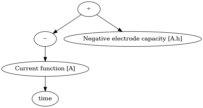

You can also print the expression as a string using the print method:

print(model.rhs[x_n])

-Current function [A] / Negative electrode capacity [A.h]

So you can see that the expression tree is a symbolic representation of the mathematical equation, which can then be later on used by the PyBaMM solvers to solve the model equations over time.

The variable children returns a list of the children nodes of a given parent node. For example, to access the Negative electrode capacity parameter we could type

model.rhs[x_n].children[1]

as it is the second children of the division node (remember python starts indexing at 0). The command can be used recursively to navigate across the expression tree. For example, if we want to access the time variable in the expression tree above, we can type

model.rhs[x_n].children[0].children[0].children[0]

This is extremely useful to debug the expression tree as it allows you to access the relevant nodes.

PyBaMM events

An event is a condition that can be used to stop the solver, for example when the voltage reaches a certain value. In PyBaMM an event can be defined using the pybamm.Event class. For example, if you wanted to define an event that stops the solver when the time reaches 3, you would write

stop_at_t_equal_3 = pybamm.Event("Stop at t = 3", pybamm.t - 3)

The expression pybamm.t - 3 is the condition that the event is looking for, and the solver will stop when this expression reaches zero. Note that the expression must evaluate to a non-negative number for the duration of the simulation, and then become zero when the event is triggered.

You can add a list of events to the model using the events attribute, the simulation will stop when any of the events are triggered.

model.events = [stop_at_t_equal_3]

Define the stochiometry cut-off events

Define four events that ensure that the stochiometries

x_n

and

x_p

are between 0 and 1. The simulation should stop when either reach 0 or 1.

PyBaMM parameter values

The final thing we need to do before we can solve the model is to define the values for all the parameters. You should already be familar with the PyBaMM pybamm.ParameterValues class, which is used to define the values of the parameters in the model. For example, if you wanted to define a parameter value for the parameter "a" that we defined earlier, you would write

parameter_values = pybamm.ParameterValues({"a": 1})

For function paramters, we can define the function using a standard Python function or lambda function that takes the same number of arguments as the function parameter. For example, if you wanted to define a function parameter for the current that is a function of time, you would write

def current(t):
    return 2 * t
parameter_values = pybamm.ParameterValues({"Current function [A]": current})

or using a lambda function

parameter_values = pybamm.ParameterValues({"Current function [A]": lambda t: 2 * t})

Define the parameter values for the reservoir model

Define the parameter values for the reservoir model. You can choose any values you like for the parameters, but in the solution below we will define the following values:

The current is a function of time, $I(t) = 1 + 0.5 \sin(100t)$
The initial negative electrode stochiometry is 0.9
The initial positive electrode stochiometry is 0.1
The negative electrode capacity is 1 Ah
The positive electrode capacity is 1 Ah
The electrode resistance is 0.1 Ohm
The OCV functions are the LGM50 OCP from the Chen2020 model, which are given by the functions:

import numpy as np
def graphite_LGM50_ocp_Chen2020(sto):
    u_eq = (
        1.9793 * np.exp(-39.3631 * sto)
        + 0.2482
        - 0.0909 * np.tanh(29.8538 * (sto - 0.1234))
        - 0.04478 * np.tanh(14.9159 * (sto - 0.2769))
        - 0.0205 * np.tanh(30.4444 * (sto - 0.6103))
    )

    return u_eq

def nmc_LGM50_ocp_Chen2020(sto):
    u_eq = (
        -0.8090 * sto
        + 4.4875
        - 0.0428 * np.tanh(18.5138 * (sto - 0.5542))
        - 17.7326 * np.tanh(15.7890 * (sto - 0.3117))
        + 17.5842 * np.tanh(15.9308 * (sto - 0.3120))
    )

    return u_eq

param = pybamm.ParameterValues({
    "Current function [A]": lambda t: 1 + 0.5 * pybamm.sin(100*t),
    "Initial negative electrode stochiometry": 0.9,
    "Initial positive electrode stochiometry": 0.1,
    "Negative electrode capacity [A.h]": 1,
    "Positive electrode capacity [A.h]": 1,
    "Electrode resistance [Ohm]": 0.1,
    "Positive electrode OCV": nmc_LGM50_ocp_Chen2020,
    "Negative electrode OCV": graphite_LGM50_ocp_Chen2020,
})

Solving the model

Now that we have defined the reservoir model, we can solve it using the PyBaMM simulation class and plot the results like so:

sim = pybamm.Simulation(model, parameter_values=param)
sol = sim.solve([0, 1])
sol.plot(["Voltage [V]", "Negative electrode stochiometry", "Positive electrode stochiometry"])

Solve the reservoir model

Solve the reservoir model using the parameter values you defined earlier, and plot the results. Vary the paramters and see how the solution changes to assure yourself that the model is working as expected.