Introduction to Hybrid Parallelism
At this point in the lesson, we've introduced the basics you need to get out there and start writing parallel code using
OpenMP. There is one thing still worth being brought to your attention, and that is hybrid parallelism.
The Message Passing Interface (MPI)
In this episode, we will assume you have some knowledge about the Message Passing Interface (MPI) and that you have a
basic understanding of how to parallelise code using MPI. If you're not sure, you can think of MPI as being like an OpenMP
program where everything is in a
pragma omp parallel directive.What is hybrid parallelism?
When we talk about hybrid parallelism, what we're really talking about is writing parallel code using more than one
parallelisation paradigm. The reason we want to do this is to take advantage of the strengths of each paradigm to
improve the performance, scaling and efficiency of our parallel core. The most common form of hybrid parallelism in
research is MPI+X. What this means is that an application is mostly parallelised using the Message Passing Interface
(MPI), which has been extended using some +X other paradigm. A common example of +X is OpenMP, creating MPI+OpenMP.
Heterogeneous Computing
An MPI+OpenMP scheme is known as homogenous computing, meaning all the processing units involved are of the same type.
The opposite is heterogeneous computing, where different types of processing architectures are used such as CPUs,
GPUs (graphics processing units), TPUs (tensor processing units) and FGPAs (field-programmable gate arrays). The goal
of heterogeneous computing is to leverage the strengths of each processor type to achieve maximum performance and
efficiency. The most common in research will be CPU and GPU.
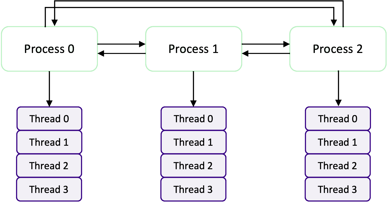
In an MPI+OpenMP application, one or multiple MPI processes/ranks are created each of which spawn their own set of
OpenMP threads as shown in the diagram above. The key thing to realise is that by combining MPI and OpenMP, we can scale
an OpenMP program from only being able to use the resources on a single HPC compute node to being able to use multiple
compute nodes. We can think of it was MPI being in charge of parallelising a program across nodes, whilst OpenMP is
responsible for the parallelism on a node.
The MPI processes are able to communicate data with one another and the threads within the same MPI process
are still using shared-memory, so do not need to communicate data. However, threads in other MPI processes cannot use
the data that threads in another MPI process have access to due to each MPI process having its own memory space. It is
still possible to communicate thread-to-thread, but we have to be very careful and explicitly set up communication
between specific threads using the parent MPI processes.
As an example of how resources could be split using an MPI+OpenMP approach, consider an HPC cluster with some number of
compute nodes with each having 64 CPU cores. One approach would be to spawn one MPI process per rank which spawns 64
OpenMP threads, or 2 MPI processes which both spawn 32 OpenMP threads, and so on and so forth.
Advantages
Improved memory efficiency
Since MPI processes each have their own private memory space, there is almost always some data replication. This could be
on small pieces of data, such as some physical constants each MPI rank needs, or it could be large pieces of data such a
grid of data or a large dataset. When there is large data being replicated in each rank, the memory requirements of an
MPI program can rapidly increase making it unfeasible to run on some systems. In an OpenMP application, we don't have to
worry about this as the threads share the same memory space and so there is no need for data replication. A huge
advantage of MPI+OpenMP is not having to replicate as much data, because there are less MPI ranks which require
replicated data.
Improved scaling and load balancing
With MPI, we can scale our OpenMP applications and use resources on multiple nodes rather than being limited to only the
resources on a single node. The advantage here is obvious. But by using OpenMP to handle the parallelism on a node, we
can more easily control the work balance, in comparison to a pure MPI implementation at least, as we can use OpenMP's
schedulers to address imbalance on a node. There is typically also a reduction in communication overheads, as there is
no communication required between threads (although this overhead may be replaced by thread synchronisation overheads)
which can improve the performance of algorithms which previously required communication such as those which require
exchanging data between overlapping subdomains (halo exchange).
Disadvantages
More difficult to write and maintain
Writing correct and efficient parallel code in pure MPI and pure OpenMP is hard enough, so combining both of them is,
naturally, even more difficult to write and maintain. Most of the difficulty comes from having to combine both
parallelism models in an easy-to-read and maintainable fashion, as the interplay between the two parallelism models adds
complexity to the code we write. We also have to ensure we do not introduce any race conditions, making sure to
synchronise threads and ranks correctly and at the correct parts of the program. Finally, because we are using two
parallelism models, MPI+OpenMP code bases are larger than a pure MPI or OpenMP version, making the overall
maintainability more challenging.
Increased overheads
Most implementations of a hybrid scheme will be slower than a pure implementation. This derives from additional
overheads, either from introducing MPI communication or from now having to worry about thread synchronisation. The
combination of coordinating and synchronisation between MPI processes and OpenMP threads increases the overheads
required to enable hybrid parallelism.
Limited portability
The portability for an MPI+OpenMP application is usually more limited, as there are more libraries and compiler versions
to consider which have to be tested for compatibility. For example, we may need to account for compiler-specific
directives for OpenMP and ensure that different MPI implementations and versions (as well as OpenMP) are compatible.
Most of this can, however, be mitigated with good documentation and a robust build system.
When do I need to use hybrid parallelism?
So, when should we use a hybrid scheme? A hybrid scheme is particularly beneficial in scenarios where you need to
leverage the strength of both the shared and distributed-memory parallelism paradigms. MPI is used to exploit lots of
resources across nodes on an HPC cluster, whilst OpenMP is used to efficiently (and somewhat easily) parallelise the work
each MPI task is required to do.
The most common reason for using a hybrid scheme is for large-scale simulations, where the workload doesn't fit or work
efficiently in a pure MPI or OpenMP implementation. This could be because of memory constraints due to data replication,
or due to poor/complex workload balance which are difficult to handle in MPI, or because of inefficient data access
patterns from how ranks are coordinated. Of course, your mileage may vary, and it is not always appropriate to use a
hybrid scheme. It could be better to think about other ways or optimisations to decrease overheads and memory
requirements, or to take a different approach to improve the work balance.
Writing a hybrid parallel application
To demonstrate how to use MPI+OpenMP, we are going to write a program which computes an approximation for using a
Riemann sum. This is not a great example to extol the virtues of hybrid
parallelism, as it is only a small problem. However, it is a simple problem which can be easily extended and
parallelised. Specifically, we will write a program to solve the integral to compute the value of ,
There are a plethora of methods available to numerically evaluate this integral. To keep the problem simple, we will
re-cast the integral into an easier-to-code summation. How we got here isn't that important for our purposes, but what we
will be implementing in code is the following summation,
where is the midpoint of the -th rectangle. To get an accurate approximation of , we'll need to
split the domain into a large number of smaller rectangles.
A simple parallel implementation using OpenMP
To begin, let's first write a serial implementation as in the code example below.
#include <stdio.h> #include <time.h> #include <unistd.h> #define PI 3.141592653589793238462643 int main(void) { struct timespec begin; clock_gettime(CLOCK_MONOTONIC_RAW, &begin); /* Initialise parameters. N is the number of rectangles we will sum over, and h is the width of each rectangle (1 / N) */ const long N = (long)1e10; const double h = 1.0 / N; double sum = 0.0; /* Compute the summation. At each iteration, we calculate the position x_i and use this value in 4 / (1 + x * x). We are not including the 1 / n factor, as we can multiply it once at the end to the final sum */ for (long i = 0; i <= N; ++i) { const double x = h * (double)i; sum += 4.0 / (1.0 + x * x); } /* To attain our final value of pi, we multiply by h as we did not include this in the loop */ const double pi = h * sum; struct timespec end; clock_gettime(CLOCK_MONOTONIC_RAW, &end); printf("Calculated pi %18.6f error %18.6f\n", pi, pi - PI); printf("Total time = %f seconds\n", (end.tv_nsec - begin.tv_nsec) / 1000000000.0 + (end.tv_sec - begin.tv_sec)); return 0; }
In the above, we are using rectangles. Although this number of rectangles is overkill, it is used to
demonstrate the performance increases from parallelisation. If we save this (as
pi.c), compile and run we should get
output as below,gcc pi.c -o pi.exe ./pi.exe Calculated pi 3.141593 error 0.000000 Total time = 34.826832 seconds
You should see that we've computed an accurate approximation of , but it also took a very long time at 35 seconds!
To speed this up, let's first parallelise this using OpenMP. All we need to do, for this simple application, is to use a
parallel for to split the loop between OpenMP threads as shown below./* Parallelise the loop using a `parallel for` directive. We will set the sum variable to be a reduction variable. As it is marked explicitly as a reduction variable, we don't need to worry about any race conditions corrupting the final value of sum */ #pragma omp parallel for shared(N, h), reduction(+:sum) for (long i = 0; i <= N; ++i) { const double x = h * (double)i; sum += 4.0 / (1.0 + x * x); } /* For diagnostics purposes, we are also going to print out the number of threads which were spawned by OpenMP */ printf("Calculated using %d OMP threads\n", omp_get_max_threads());
Once we have made these changes (you can find the completed implementation here), compiled
and run the program, we can see there is a big improvement to the performance of our program. It takes just 5 seconds to
complete, instead of 35 seconds, to get our approximate value of , e.g.:
gcc -fopenmp pi-omp.c -o pi.exe ./pi.exe Calculated using 8 OMP threads Calculated pi 3.141593 error 0.000000 Total time = 5.166490 seconds
A hybrid implementation using MPI and OpenMP
Now that we have a working parallel implementation using OpenMP, we can now expand our code to a hybrid parallel code by
implementing MPI. In this example, we wil be porting an OpenMP code to a hybrid MPI+OpenMP application, but we could have
also done this the other way around by porting an MPI code into a hybrid application. Neither "evolution" is more
common nor better than the other, the route each code takes toward becoming hybrid is different.
So, how do we split work using a hybrid approach? For an embarrassingly parallel problem, such as the one we're working on,
we can split the problem size into smaller chunks across MPI ranks and use OpenMP to parallelise the work. For example, consider
a problem where we have to do a calculation for 1,000,000 input parameters. If we have four MPI ranks each of which will spawn 10 threads,
we could split the work evenly between MPI ranks so each rank will deal with 250,000 input parameters. We will then use OpenMP
threads to do the calculations in parallel. If we use a sequential scheduler, then each thread will do 25,000 calculations. Or we
could use OpenMP's dynamic scheduler to automatically balance the workload. We have implemented this situation in the code example below.
/* We have an array of input parameters. The calculation which uses these parameters is expensive, so we want to split them across MPI ranks */ struct input_par_t input_parameters[total_work]; /* We need to determine how many input parameters each rank will process (we are assuming total_work is cleanly divisible) and also lower and upper indices of the input_parameters array the rank will work on */ int work_per_rank = total_work / num_ranks; int rank_lower_limit = my_rank * work_per_rank; int rank_upper_limit = (my_rank + 1) * work_per_rank; /* The MPI rank now knows which subset of data it will work on, but we will use OpenMP to spawn threads to execute the calculations in parallel. We'll make sure of the auto scheduler to best determine how to balance the work */ #pragma omp parallel for schedule(auto) for (int i = rank_lower_limit; i < rank_upper_limit; ++i) { some_expensive_calculation(input_parameters[i]); }
Still not sure about MPI?
If you're still a bit unsure of how MPI is working, you can basically think of it as wrapping large parts of your
code in a
pragma omp parallel region as we saw in an earlier episode. We can re-write the code example above in the
same way, but using OpenMP thread IDs instead.struct input_par_t input_parameters[total_work]; #pragma omp parallel { int num_threads = omp_get_num_threads(); int thread_id = omp_get_thread_num(); int work_per_thread = total_work / num_threads; int thread_lower = thread_id * work_per_thread; int thread_upper = (thread_id + 1) * work_per_thread; for(int i = thread_lower; i < thread_upper; ++i) { some_expensive_calculation(input_parameters[i]); } }
In the above example, we have only included the parallel region of code. It is unfortunately not as simple as this,
because we have to deal with the additional complexity from using MPI. We need to initialise MPI, as well as communicate
and receive data and deal with the other complications which come with MPI. When we include all of this, our code
example becomes much more complicated than before. In the next code block, we have implemented a hybrid MPI+OpenMP
approximation of using the same Riemann sum method.
#include <stdlib.h> #include <stdio.h> #include <time.h> #include <unistd.h> #include <mpi.h> #include <omp.h> #define PI 3.141592653589793238462643 #define ROOT_RANK 0 int main(void) { struct timespec begin; clock_gettime(CLOCK_MONOTONIC_RAW, &begin); /* We have to initialise MPI first and determine the number of ranks and which rank we are to be able to split work with MPI */ int my_rank; int num_ranks; MPI_Init(NULL, NULL); MPI_Comm_rank(MPI_COMM_WORLD, &my_rank); MPI_Comm_size(MPI_COMM_WORLD, &num_ranks); /* We can leave this part unchanged, the parameters per rank will be the same */ double sum = 0.0; const long N = (long)1e10; const double h = 1.0 / N; /* The OpenMP parallelisation is almost the same, we are still using a parallel for to do the loop in parallel. To parallelise using MPI, we have each MPI rank do every num_rank-th iteration of the loop. Each rank will do N / num_rank iterations split between it's own OpenMP threads */ #pragma omp parallel for shared(N, h, my_rank, num_ranks), reduction(+:sum) for (long i = my_rank; i <= N; i = i + num_ranks) { const double x = h * (double)i; sum += 4.0 / (1.0 + x * x); } /* The sum we compute is per rank now, but only includes N / num_rank elements so is not the final value of pi */ const double rank_pi = h * sum; /* To get the final value, we will use a reduction across ranks to sum up the contributions from each MPI rank */ double reduced_pi; MPI_Reduce(&rank_pi, &reduced_pi, 1, MPI_DOUBLE, MPI_SUM, 0, MPI_COMM_WORLD); if (my_rank == ROOT_RANK) { struct timespec end; clock_gettime(CLOCK_MONOTONIC_RAW, &end); /* Let's check how many ranks are running and how many threads each rank is spawning */ printf("Calculated using %d MPI ranks each spawning %d OMP threads\n", num_ranks, omp_get_max_threads()); printf("Calculated pi %18.6f error %18.6f\n", reduced_pi, reduced_pi - PI); printf("Total time = %f seconds\n", (end.tv_nsec - begin.tv_nsec) / 1000000000.0 + (end.tv_sec - begin.tv_sec)); } MPI_Finalize(); return 0; }
So you can see that it's much longer and more complicated; although not much more than a pure MPI
implementation. To compile our hybrid program, we use the MPI compiler command
mpicc with
the argument -fopenmp. We can then run our compiled program using mpirun.mpicc -fopenmp 05-pi-omp-mpi.c -o pi.exe mpirun pi.exe Calculated 8 MPI ranks each spawning 8 OMP threads Calculated pi 3.141593 error 0.000000 Total time = 5.818889 seconds
Ouch, this took longer to run than the pure OpenMP implementation (although only marginally longer in this example!). You
may have noticed that we have 8 MPI ranks, each of which are spawning 8 of their own OpenMP threads. This is an
important thing to realise. When you specify the number of threads for OpenMP to use, this is the number of threads
each MPI process will spawn. So why did it take longer? With each of the 8 MPI ranks spawning 8 threads, 64 threads
were in flight. More threads means more overheads and if, for instance, we have 8 CPU Cores, then contention
arises as each thread competes for access to a CPU core.
Let's improve this situation by using a combination of rank and threads so that . One way to do this is by setting the
OMP_NUM_THREADS environment variable and by specifying the number of
processes we want to spawn with mpirun. For example, we can spawn two MPI processes which will both spawn 4 threads
each.export OMP_NUM_THREADS 4 mpirun -n 2 pi.exe Calculated using 4 OMP threads and 2 MPI ranks Calculated pi 3.141593 error 0.000000 Total time = 5.078829 seconds
This is better now, as threads aren't fighting for access to a CPU core. If we change the number of ranks to 1 and
the number of threads to 8, will it take the same amount of time to run as the pure OpenMP implementation?
export OMP_NUM_THREADS 8 mpirun -n 1 pi.exe Calculated using 8 OMP threads and 1 MPI ranks Calculated pi 3.141593 error 0.000000 Total time = 5.328421 seconds
In this case, we don't. It takes slightly longer to run because of the overhead associated with MPI. Even when we use
one MPI rank, we still have to initialise MPI, set the rank number, and so on. All of this takes time. The same happens
with using 8 ranks and 1 thread per rank, as there is still a slight overhead related to scheduling the work for that
single OpenMP thread.
export OMP_NUM_THREADS 1 mpirun -n 8 pi.exe Calculated using 1 OMP threads and 8 MPI ranks Calculated pi 3.141593 error 0.000000 Total time = 5.377609 seconds
How many ranks and threads should I use?
How many ranks and threads you should use depends on lots of parameters, such as the size of your problem (e.g. do you
need a large number of threads but a smaller number of ranks to improve memory efficiency?), the hardware you are
using and the design/structure of your code. It's unfortunately very difficult to predict the best combination of
ranks and threads. Often we won't know until after we've run lots of tests and gained some intuition. It's a
delicate balance of balancing overheads associated with thread synchronisation in OpenMP and data communication in
MPI. As mentioned earlier, a hybrid implementation will typically be slower than a "pure" MPI implementation for example.
Optimum combination of threads and ranks for approximating Pi
Note that there will be some level of variance in the run time each time you run the program, due to factors such as
other programs using your CPU at the same time. You should run each thread/rank combination multiple time to get an
average.